Lab: Eigenvalues in Action (Webpage Navigation and PCA)

linear-algebra

In this lab you will apply eigenvalues and eigenvectors to two real-world problems: modeling how users navigate between webpages (Markov chains), and…

Published

June 6, 2026

In this lab you will apply eigenvalues and eigenvectors to two real-world problems: modeling how users navigate between webpages (Markov chains), and reducing the dimensionality of image data using PCA.

Setup

import numpy as np
import matplotlib.pyplot as plt

%config InlineBackend.figure_formats = ['png']
np.random.seed(42)

Part 1: Navigating Webpages with Markov Chains

Consider a small internet with 5 pages. Each page links to some others, and a user clicks links randomly. The probability of moving from page \(j\) to page \(i\) is stored in a transition matrix \(P\) where each column sums to 1.

Building the Transition Matrix

P = np.array([
    [0,    0.75, 0.35, 0.25, 0.85],
    [0.15, 0,    0.35, 0.25, 0.05],
    [0.15, 0.15, 0,    0.25, 0.05],
    [0.15, 0.05, 0.05, 0,    0.05],
    [0.55, 0.05, 0.25, 0.25, 0]
])

print("Transition matrix P:")
print(P)
print(f"\nColumn sums (should all be 1): {P.sum(axis=0)}")

Transition matrix P:
[[0.   0.75 0.35 0.25 0.85]
 [0.15 0.   0.35 0.25 0.05]
 [0.15 0.15 0.   0.25 0.05]
 [0.15 0.05 0.05 0.   0.05]
 [0.55 0.05 0.25 0.25 0.  ]]

Column sums (should all be 1): [1. 1. 1. 1. 1.]

Each column represents “if the user is on page \(j\), what are the probabilities of going to each page next?” For example, column 1 says: from page 1, there’s a 75% chance of going to page 2, 15% to page 3, etc.

One Step of Navigation

If the user starts on page 1 with certainty, the initial state is:

X0 = np.array([[1], [0], [0], [0], [0]])
print("Initial state (on page 1):")
print(X0.flatten())

# After one click:
X1 = P @ X0
print(f"\nAfter 1 step:\n{X1.flatten()}")

Initial state (on page 1):
[1 0 0 0 0]

After 1 step:
[0.   0.15 0.15 0.15 0.55]

Many Steps: Converging to Equilibrium

Let’s iterate many times and watch the state vector stabilize:

X = X0.copy()
history = [X.flatten()]

for i in range(30):
    X = P @ X
    history.append(X.flatten())

history = np.array(history)

fig, ax = plt.subplots(1, 1, figsize=(8, 5))
for page in range(5):
    ax.plot(history[:, page], '-o', markersize=3, label=f'Page {page+1}')
ax.set_xlabel('Steps', fontsize=11)
ax.set_ylabel('Probability', fontsize=11)
ax.set_title('State vector converges to equilibrium', fontsize=12, color='gray')
ax.legend(fontsize=10)
ax.grid(True, linestyle='--', alpha=0.4)
plt.tight_layout()
plt.show()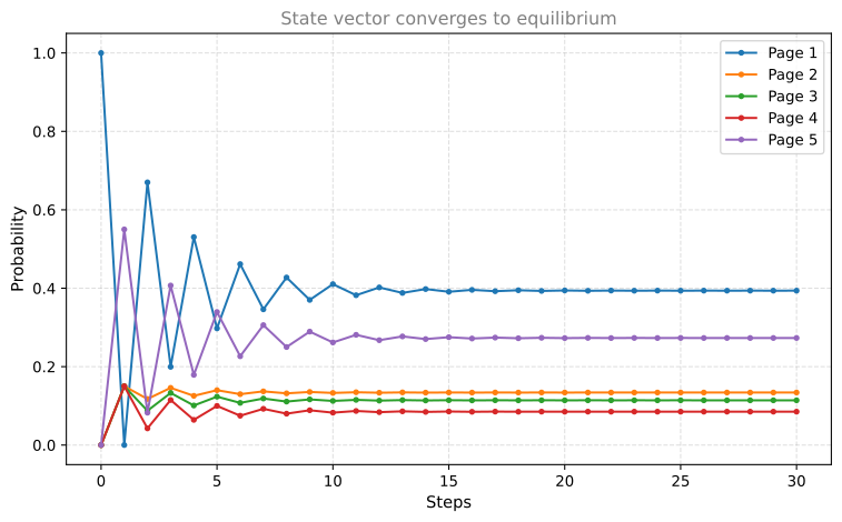

After enough steps, the probabilities stabilize. This is the equilibrium state.

Finding the Equilibrium with Eigenvalues

The equilibrium state is the eigenvector of \(P\) with eigenvalue 1:

eigenvalues, eigenvectors = np.linalg.eig(P)

print("Eigenvalues:")
for i, val in enumerate(eigenvalues):
    print(f"  λ_{i+1} = {val:.4f}")

Eigenvalues:
  λ_1 = 1.0000
  λ_2 = -0.7037
  λ_3 = 0.0054
  λ_4 = -0.0827
  λ_5 = -0.2191

# Find the eigenvector with eigenvalue closest to 1
idx = np.argmin(np.abs(eigenvalues - 1.0))
X_inf = eigenvectors[:, idx].real

# Normalize so entries sum to 1 (probability distribution)
X_inf = X_inf / X_inf.sum()

print(f"Equilibrium state (eigenvector with λ=1, normalized):")
for i, p in enumerate(X_inf):
    print(f"  Page {i+1}: {p:.4f} ({p*100:.1f}%)")

Equilibrium state (eigenvector with λ=1, normalized):
  Page 1: 0.3938 (39.4%)
  Page 2: 0.1339 (13.4%)
  Page 3: 0.1141 (11.4%)
  Page 4: 0.0851 (8.5%)
  Page 5: 0.2731 (27.3%)

Verification

Let’s verify: multiplying the equilibrium vector by \(P\) should give back the same vector:

X_check = P @ X_inf.reshape(-1, 1)
print("P @ X_inf:")
print(X_check.flatten().round(4))
print(f"\nX_inf:")
print(X_inf.round(4))
print(f"\nDifference (should be ~0): {np.abs(X_check.flatten() - X_inf).max():.2e}")

P @ X_inf:
[0.3938 0.1339 0.1141 0.0851 0.2731]

X_inf:
[0.3938 0.1339 0.1141 0.0851 0.2731]

Difference (should be ~0): 5.55e-17

The page with the highest equilibrium probability gets the most long-term traffic. This is the core idea behind Google’s PageRank algorithm.

Part 2: PCA on Image Data

Now let’s apply PCA to reduce the dimensionality of image data, the classic data compression use of PCA from the machine learning notes. We’ll work with 55 grayscale cat photos (64×64 pixels each).

Load the Images

from PIL import Image
import os

# Load cat images, convert to grayscale, resize to 64x64
img_dir = '../../media/cats/'
img_size = 64

filenames = sorted([f for f in os.listdir(img_dir) if f.endswith('.jpg')],
                   key=lambda x: int(x.split('(')[1].split(')')[0]))

imgs = []
for fname in filenames:
    img = Image.open(os.path.join(img_dir, fname)).convert('L').resize((img_size, img_size))
    imgs.append(np.array(img))

imgs = np.array(imgs)
print(f"Dataset: {imgs.shape[0]} images, each {imgs.shape[1]}×{imgs.shape[2]} pixels")

Dataset: 55 images, each 64×64 pixels

# Display a few sample images
fig, axes = plt.subplots(2, 5, figsize=(12, 5))
for i, ax in enumerate(axes.flat):
    ax.imshow(imgs[i], cmap='gray')
    ax.set_title(f'Cat {i+1}', fontsize=9)
    ax.axis('off')
plt.suptitle('Sample cat images from the dataset', fontsize=12, color='gray')
plt.tight_layout()
plt.show()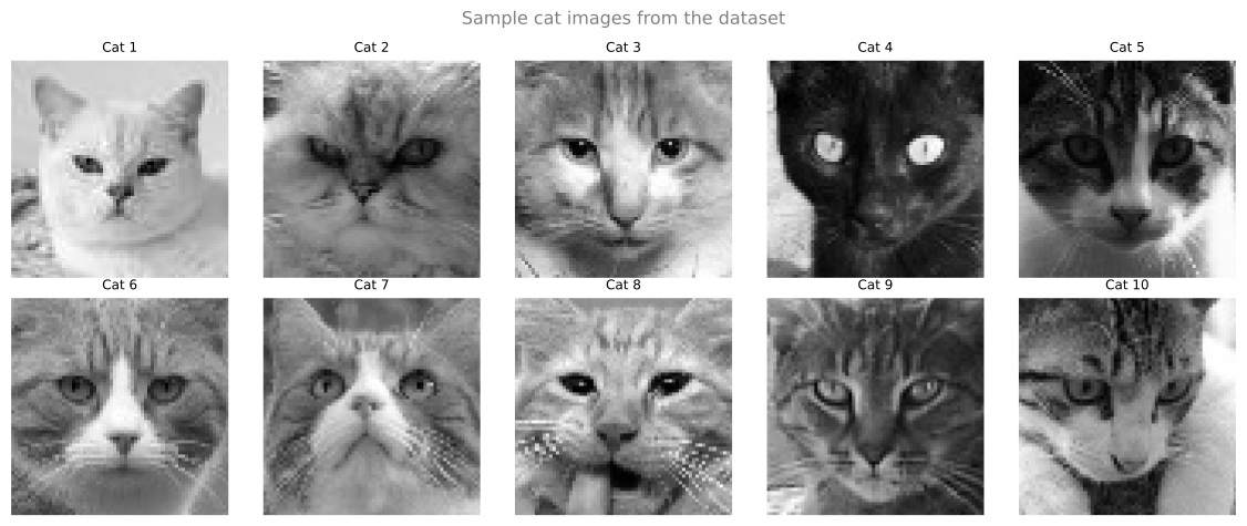

Step 1: Flatten the Images

Each 64×64 image becomes a single row vector of length 4096:

n_images = imgs.shape[0]
imgs_flatten = imgs.reshape(n_images, -1).astype(float)
print(f"Flattened shape: {imgs_flatten.shape}")
print(f"Each image is now a vector of {imgs_flatten.shape[1]} pixel values")

Flattened shape: (55, 4096)
Each image is now a vector of 4096 pixel values

Step 2: Center the Data

Subtract the mean of each pixel (column) across all images:

mean_img = imgs_flatten.mean(axis=0)
X = imgs_flatten - mean_img

print(f"Centered data shape: {X.shape}")
print(f"Column means after centering (should be ~0): {X.mean(axis=0)[:5].round(10)}")

Centered data shape: (55, 4096)
Column means after centering (should be ~0): [-0.  0.  0. -0.  0.]

Step 3: Compute the Covariance Matrix

n = X.shape[0]
C = (X.T @ X) / (n - 1)
print(f"Covariance matrix shape: {C.shape}")

Covariance matrix shape: (4096, 4096)

Step 4: Find Eigenvalues and Eigenvectors

For large matrices, we use scipy.sparse.linalg.eigs which efficiently finds only the top \(k\) eigenvalues:

from scipy.sparse.linalg import eigs

# Find top 10 eigenvalues/eigenvectors
k = 10
eigenvalues, eigenvectors = eigs(C, k=k)
eigenvalues = eigenvalues.real
eigenvectors = eigenvectors.real

# Sort by eigenvalue (largest first)
idx = np.argsort(-eigenvalues)
eigenvalues = eigenvalues[idx]
eigenvectors = eigenvectors[:, idx]

print("Top 10 eigenvalues:")
for i, val in enumerate(eigenvalues):
    print(f"  PC{i+1}: λ = {val:.1f} ({val/eigenvalues.sum()*100:.1f}% of top-10 variance)")

Top 10 eigenvalues:
  PC1: λ = 4331856.2 (34.4% of top-10 variance)
  PC2: λ = 2482088.6 (19.7% of top-10 variance)
  PC3: λ = 1546805.6 (12.3% of top-10 variance)
  PC4: λ = 1001483.1 (8.0% of top-10 variance)
  PC5: λ = 860323.6 (6.8% of top-10 variance)
  PC6: λ = 823820.2 (6.5% of top-10 variance)
  PC7: λ = 463460.4 (3.7% of top-10 variance)
  PC8: λ = 414722.6 (3.3% of top-10 variance)
  PC9: λ = 372742.9 (3.0% of top-10 variance)
  PC10: λ = 297975.5 (2.4% of top-10 variance)

Step 5: Visualize Principal Components

Each eigenvector (principal component) is itself a 4096-length vector that can be reshaped back into a 64×64 image:

fig, axes = plt.subplots(2, 5, figsize=(12, 5))
for i, ax in enumerate(axes.flat):
    pc_img = eigenvectors[:, i].reshape(img_size, img_size)
    ax.imshow(pc_img, cmap='gray')
    ax.set_title(f'PC{i+1}', fontsize=9)
    ax.axis('off')
plt.suptitle('Top 10 principal components (eigenvectors as images)', fontsize=12, color='gray')
plt.tight_layout()
plt.show()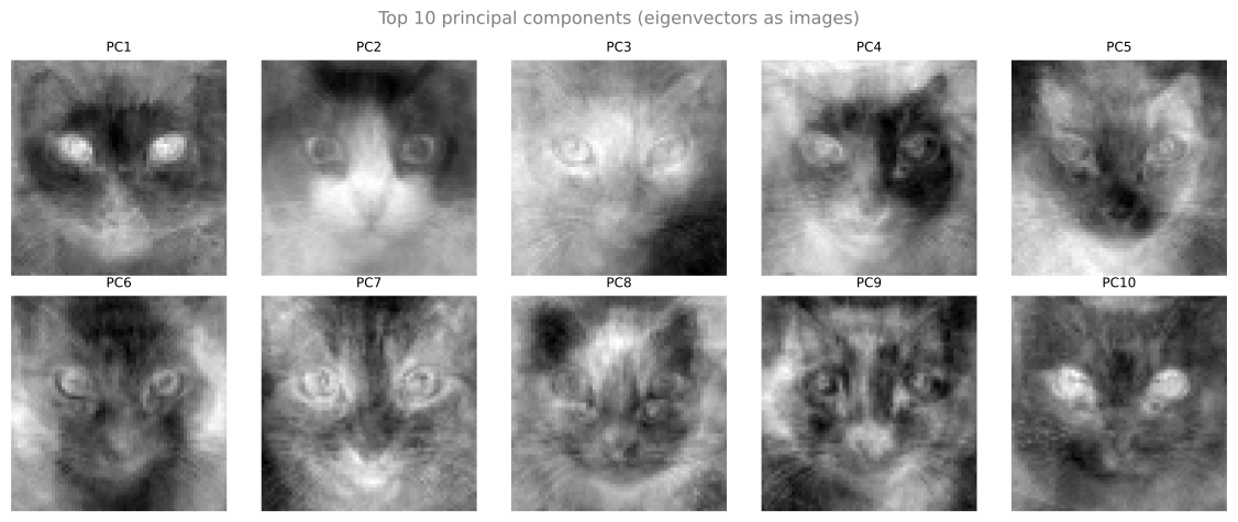

Step 6: Project and Reduce Dimensions

Project all images onto the top 2 principal components:

def pca_transform(X, eigenvectors, n_components):
    """Project centered data onto top n principal components."""
    V = eigenvectors[:, :n_components]
    return X @ V

# Reduce to 2 dimensions
X_2d = pca_transform(X, eigenvectors, 2)
print(f"Original: {X.shape[1]} dimensions → Reduced: {X_2d.shape[1]} dimensions")

Original: 4096 dimensions → Reduced: 2 dimensions

fig, ax = plt.subplots(1, 1, figsize=(7, 6))
ax.scatter(X_2d[:, 0], X_2d[:, 1], s=40, color='#4682B4', alpha=0.7)
for i in range(n_images):
    ax.annotate(str(i+1), (X_2d[i, 0]+0.5, X_2d[i, 1]+0.5), fontsize=7, alpha=0.6)
ax.set_xlabel('PC1', fontsize=11)
ax.set_ylabel('PC2', fontsize=11)
ax.set_title('All images projected onto 2 principal components', fontsize=12, color='gray')
ax.grid(True, linestyle='--', alpha=0.4)
plt.tight_layout()
plt.show()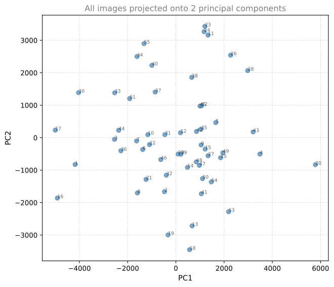

Images that appear close together in this 2D plot are similar in the original 4096-dimensional space.

Step 7: Reconstruction

You can approximately reconstruct an image from its reduced representation:

fig, axes = plt.subplots(2, 4, figsize=(12, 6))
components_list = [1, 2, 5, 10]
img_idx = 0

for i, n_comp in enumerate(components_list):
    V = eigenvectors[:, :n_comp]
    projected = X[img_idx] @ V        # reduce
    reconstructed = projected @ V.T    # reconstruct
    reconstructed += mean_img          # add mean back

    axes[0, i].imshow(reconstructed.reshape(img_size, img_size), cmap='gray')
    axes[0, i].set_title(f'{n_comp} components', fontsize=10)
    axes[0, i].axis('off')

axes[1, 0].imshow(imgs[img_idx], cmap='gray')
axes[1, 0].set_title('Original', fontsize=10)
axes[1, 0].axis('off')
for ax in axes[1, 1:]:
    ax.axis('off')

plt.suptitle(f'Reconstructing image {img_idx+1} with different numbers of components', fontsize=12, color='gray')
plt.tight_layout()
plt.show()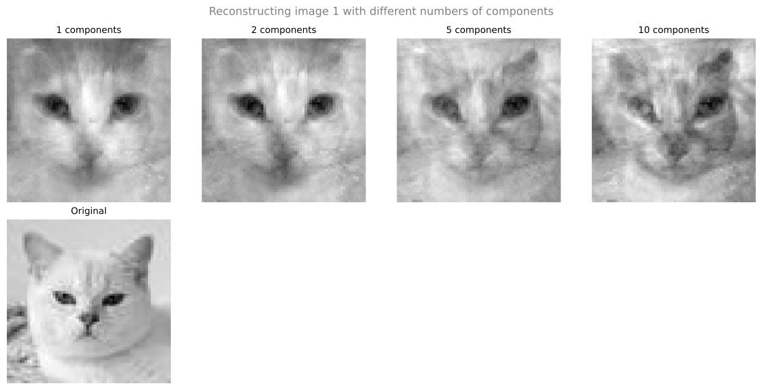

With more principal components, the reconstruction gets closer to the original. Even a few components capture the main structure.

Key Takeaway

The full PCA pipeline:

Flatten images to vectors (64×64 → 4096)
Center the data (subtract mean)
Compute covariance matrix (\(4096 \times 4096\))
Find top \(k\) eigenvectors
Project: \(X_{\text{reduced}} = X \cdot V_k\) (4096 → \(k\) dimensions)
Reconstruct: \(X_{\text{approx}} = X_{\text{reduced}} \cdot V_k^T + \mu\)

You reduced 4096 pixel values to just a handful of numbers, while keeping the essential structure of each image.