Systems of Equations
linear-algebra
The first topic you learn in linear algebra is systems of linear equations. However, before you delve into equations, it is important to understand the…
Systems of Sentences
The first topic you learn in linear algebra is systems of linear equations. However, before you delve into equations, it is important to understand the language of mathematics. When I think of equations, I think of sentences. Sentences that are giving you information about things in the world. Systems of sentences behave a lot like systems of equations as you’ll see in the following example.
So let’s start with some examples of systems of sentences. Now, for the sake of this example, assume that you only have one dog and one cat and they’re both of only one color. You are given some information and your goal is to try to figure out the color of each of the animals.
Example with Two Sentences
System 1: The dog is black and the cat is orange.
System 2: The dog is black and the dog is black.
System 3: The dog is black and the dog is white.
The sentences here are simple sentences with one piece of information each. Sentences such as “the dog is black and the dog is white” are not allowed as they separately contain two pieces of information. The goal for a system is to convey as much information as possible with these simple sentences.
With regards to achieving that goal, notice that these systems are quite different:
- System 1 contains two sentences and two pieces of information. This means the system contains as many pieces of information as sentences and that’s called a complete system.
- System 2 is a bit less informative as it has two sentences, but they’re exactly the same. Therefore the system only carries one piece of information even though it contains two sentences. The sentences repeat themselves and therefore the system is called redundant.
- System 3 is strange as the sentences contradict each other. This is because the dog can’t be black and white at the same time (remember that we have one dog and it can only have one color). So the system is called contradictory.
Terminology: Singular vs Non-Singular Systems
The more information a system carries, the more useful it will be for you. For this reason we’ll introduce some terminology that you’ll be using throughout the whole course:
- When a system is redundant or contradictory, it’s called a singular system.
- When a system is complete, it’s called a non-singular system.
In a nutshell, a non-singular system is a system that carries as many pieces of information as sentences. So it’s the most informative system can be, and a singular system is less informative than a non-singular one.
| System 1 | System 2 | System 3 |
|---|---|---|
| The dog is black | The dog is black | The dog is black |
| The cat is orange | The dog is black | The dog is white |
| Complete | Redundant | Contradictory |
| Non-Singular | Singular | Singular |
Example with More Sentences
Systems of sentences can carry more than two sentences. In fact they can carry as many as we want. Here are some examples of systems with three sentences. In this new example, you have three animals and are again trying to determine their color:
System 1: The dog is black, the cat is orange and the bird is red.
System 2: The dog is black, the dog is black and the bird is red.
System 3: The dog is black, the dog is black and the dog is black.
System 4: The dog is black, the dog is white and the bird is red.
Analyzing these systems:
- System 1 is complete as it carries three different pieces of information using three sentences, so it’s complete and non-singular.
- System 2 is redundant and singular as the 1st and 2nd sentences say the exact same thing.
- System 3 is redundant as all the sentences say the same thing.
- System 4 is contradictory because the dog can’t be black and white at the same time.
Notice that System 3 is more redundant than System 2. Is there a measure of how redundant a system is? The answer is yes, and it’s called rank. The rank of a system is the number of pieces of information it carries. So System 1 has rank 3, System 2 has rank 2, System 3 has rank 1, and System 4 has rank 2. The higher the rank, the more informative the system is.
| System 1 | System 2 | System 3 | System 4 |
|---|---|---|---|
| The dog is black | The dog is black | The dog is black | The dog is black |
| The cat is orange | The dog is black | The dog is black | The dog is white |
| The bird is red | The bird is red | The dog is black | The bird is red |
| Complete | Redundant | Redundant | Contradictory |
| Non-Singular | Singular | Singular | Singular |
From Sentences to Equations
Just like sentences, equations are statements that give you information. A sentence like “the price of an apple and a banana is $10” translates directly into the equation \(a + b = 10\), where \(a\) is the price of an apple and \(b\) is the price of a banana.
System 1: The Grocery Store Problem (Two Unknowns)
Imagine a peculiar grocery store where individual items don’t have price tags — you only see the total at the register. Being a math person, you keep track of totals to deduce individual prices.
- Day 1:
+ = $10 - Day 2:
+ = $12
The difference between the two days? One extra banana for $2 extra. So bananas cost $2 each. Plugging back into Day 1: the apple must cost $8.
\[\begin{cases} a + b = 10 \\ a + 2b = 12 \end{cases} \quad \Rightarrow \quad b = 2, \; a = 8\]
This system is complete and non-singular — two equations, two pieces of information, one unique solution.
System 2: Redundant System (Infinitely Many Solutions)
- Day 1:
+ = $10 - Day 2:
+ = $20
Day 2 is just Day 1 multiplied by 2 — it adds no new information. Any two prices that add to 10 work: \((8, 2)\), \((5, 5)\), \((0, 10)\), etc. The system is redundant and singular with infinitely many solutions.
\[\begin{cases} a + b = 10 \\ 2a + 2b = 20 \end{cases} \quad \Rightarrow \quad \text{infinitely many solutions}\]
System 3: Contradictory System (No Solution)
- Day 1:
+ = $10 - Day 2:
+ = $24
If \(a + b = 10\), then \(2a + 2b\) must be $20, not $24. The equations contradict each other. The system is contradictory and singular with no solution.
\[\begin{cases} a + b = 10 \\ 2a + 2b = 24 \end{cases} \quad \Rightarrow \quad \text{no solution}\]
Summary
| System | Equations | Type | Solutions |
|---|---|---|---|
| 1 | \(\begin{cases} a + b = 10 \\ a + 2b = 12 \end{cases}\) | Complete, Non-singular | Unique: \(a=8, b=2\) |
| 2 | \(\begin{cases} a + b = 10 \\ 2a + 2b = 20 \end{cases}\) | Redundant, Singular | Infinitely many |
| 3 | \(\begin{cases} a + b = 10 \\ 2a + 2b = 24 \end{cases}\) | Contradictory, Singular | None |
What Makes an Equation “Linear”?
In a linear equation, variables can only be multiplied by constants (scalars) and then added or subtracted, plus an optional constant term:
\[ \begin{array}{ll} \color{green}{3.4a - 48.99b + 2c = 122.5} & \color{green}{\text{(linear)}} \end{array} \]
Non-linear equations involve squares (\(a^2\)), products of variables (\(ab\)), trigonometric functions (\(\sin a\)), exponentials (\(2^a\)), logarithms (\(\log b\)), division by variables (\(3/b\)), etc. Linear algebra is the study of linear equations — and because they are simpler, there is a rich set of tools for manipulating them and extracting information.
\[ \begin{array}{ll} \color{red}{a^2 + b^2 = 10} & \color{red}{\text{(non-linear)}}\\ \color{red}{\sin(a) + b^5 = 15} & \color{red}{\text{(non-linear)}}\\ \color{red}{2^a - 3^b = 0} & \color{red}{\text{(non-linear)}}\\ \color{red}{ab^2 + \dfrac{b}{a} - \dfrac{3}{b} - \log(c) = 4^a} & \color{red}{\text{(non-linear)}} \end{array} \]
Systems of Linear Equations as Lines and Planes
Now that you know what a system of linear equations is and when they are singular or non-singular, it’s time for some visualizations. Linear equations in two variables can be visualized as lines in the coordinate plane. If you have three variables, they become planes in space. And with more variables, they become higher-dimensional objects.
Equations as Lines
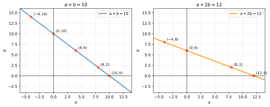
How can you visualize the equation \(a + b = 10\) as a line? Set up a grid where the horizontal axis represents \(a\) (price of an apple) and the vertical axis represents \(b\) (price of a banana). Then find pairs of numbers that add to 10:
- \((10, 0)\) because \(10 + 0 = 10\)
- \((0, 10)\) because \(0 + 10 = 10\)
- \((4, 6)\) because \(4 + 6 = 10\)
- \((8, 2)\) because \(8 + 2 = 10\)
- \((-4, 14)\) because \(-4 + 14 = 10\)
All these points form a line. Every single point on this line is a solution to the equation.
Similarly, the equation \(a + 2b = 12\) gives us another line. Some solutions: \((0, 6)\), \((12, 0)\), \((8, 2)\), \((-4, 8)\).
The slope of \(a + b = 10\) is \(-1\) (for every unit you move right, the line drops one unit). Its \(b\)-intercept is \(10\). The slope of \(a + 2b = 12\) is \(-0.5\) and its \(b\)-intercept is \(6\).
Systems as Arrangements of Lines
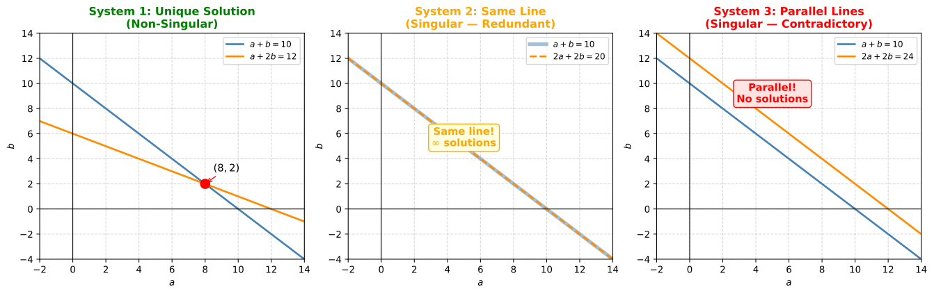
Since each equation corresponds to a line, a system of two equations corresponds to two lines in the same plane. The solution to the system is where the lines intersect.
System 1: Unique Solution (Non-Singular)
\[\begin{cases} a + b = 10 \\ a + 2b = 12 \end{cases}\]
The two lines cross at exactly one point: \((8, 2)\). This is the unique solution.
System 2: Infinitely Many Solutions (Singular — Redundant)
\[\begin{cases} a + b = 10 \\ 2a + 2b = 20 \end{cases}\]
The line \(2a + 2b = 20\) passes through the same points as \(a + b = 10\) — it’s the exact same line. The two lines overlap completely, so every point on the line is a solution.
System 3: No Solution (Singular — Contradictory)
\[\begin{cases} a + b = 10 \\ 2a + 2b = 24 \end{cases}\]
The line \(2a + 2b = 24\) passes through \((0, 12)\) and \((12, 0)\). It’s parallel to \(a + b = 10\), shifted up by 2 units. Parallel lines never meet, so there are no solutions.
Quiz: Plotting a System
Consider the system:
\[\begin{cases} 3a + 2b = 8 \\ 2a - b = 3 \end{cases}\]
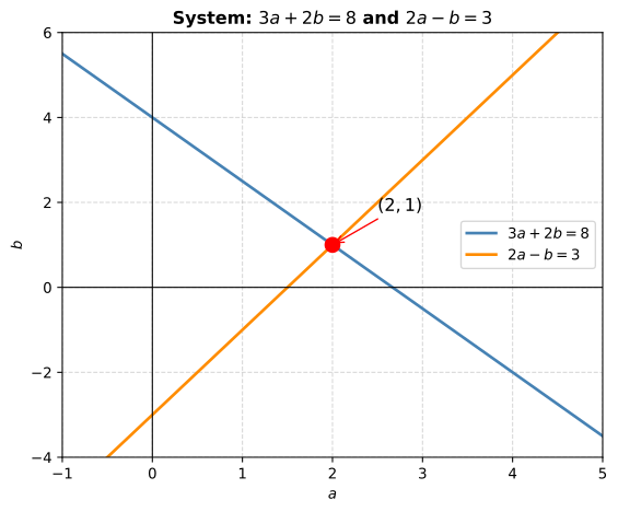
The line \(3a + 2b = 8\) passes through \((0, 4)\) and \((8/3, 0)\). The line \(2a - b = 3\) passes through \((0, -3)\) and \((3/2, 0)\). The two lines cross at \((2, 1)\), which is the unique solution. Since they intersect at one point, the system is non-singular.
Equations as Planes in 3D (3 Variables)
A linear equation in three variables corresponds to a plane in 3D space. For example, the equation \(a + b + c = 1\) passes through the points \((1,0,0)\), \((0,1,0)\), and \((0,0,1)\). Three points define a plane, and every point on that plane is a solution.
When the constant is zero (e.g., \(3a - 5b + 2c = 0\)), the plane must pass through the origin \((0,0,0)\), because \(a=0, b=0, c=0\) satisfies the equation.
Just as we intersect lines to solve systems in 2D, we intersect planes in 3D. Two planes intersect in a line. Three planes can intersect at a single point, along a line, or not at all.
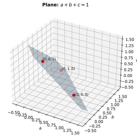
Same plane as a rotatable surface, so the three marked points can be viewed from any angle
\[\begin{cases} a + b + c = 0 \\ a + 2b + c = 0 \\ a + b + 2c = 0 \end{cases}\]
The first plane passes through the origin. The second plane also passes through the origin, and the two intersect along a line. The third plane cuts through that line at exactly one point: \((0, 0, 0)\). This is the unique solution — the system is non-singular.
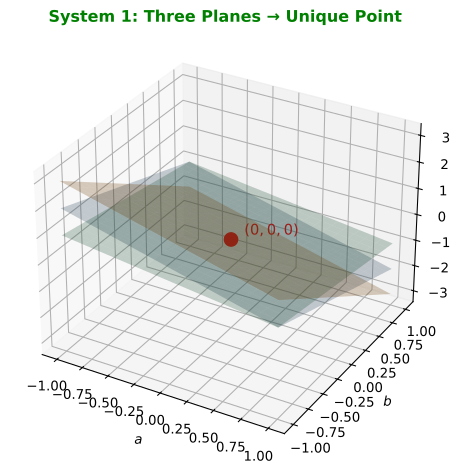
Rotatable view of the same three planes, showing the single point they share
System 2: Three Planes Share a Line (Singular — Redundant)
\[\begin{cases} a + b + c = 0 \\ a + b + 2c = 0 \\ a + b + 3c = 0 \end{cases}\]
From the first two equations, subtracting gives \(c = 0\). From the second and third, subtracting also gives \(c = 0\). So the third equation adds nothing new. All three planes pass through the origin and intersect along the line \(c = 0, \; a + b = 0\) (i.e., \(a = -b\)). The solution set is an entire line, so there are infinitely many solutions — the system is singular (redundant).
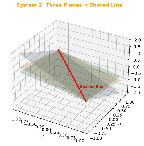
Rotatable view of the three planes intersecting along a line rather than at a point
System 3: Three Planes Are the Same Plane (Singular — Redundant)
\[\begin{cases} a + b + c = 0 \\ 2a + 2b + 2c = 0 \\ 3a + 3b + 3c = 0 \end{cases}\]
The second equation is just the first multiplied by 2, and the third is the first multiplied by 3. All three equations describe the exact same plane. Every point on that plane is a solution — infinitely many solutions. The system is singular (redundant).
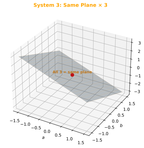
Rotatable view of the single shared plane the three equations collapse onto
For three equations in three unknowns, the same classification applies:
- Non-singular: Three planes meet at a single point → unique solution
- Singular (redundant): Planes share a common line or are the same plane → infinitely many solutions
- Singular (contradictory): Planes have no common point → no solution
Singular and Non-Singular Matrices
When determining whether a system is singular or non-singular, the constants on the right-hand side don’t matter — only the coefficients do. This means we can represent a system purely as a matrix of coefficients.
For example, the system:
\[\begin{cases} a + b + c = 10 \\ a + 2b + c = 15 \\ a + b + 2c = 12 \end{cases}\]
has the coefficient matrix:
\[\begin{bmatrix} 1 & 1 & 1 \\ 1 & 2 & 1 \\ 1 & 1 & 2 \end{bmatrix}\]
The singularity of the system depends entirely on this matrix.
Linear Dependence and Independence
A matrix is singular when one row can be obtained from the others — the rows are linearly dependent. A matrix is non-singular when no row can be obtained from the others — the rows are linearly independent.
Recall the singular system \(a + b = 10\) and \(2a + 2b = 20\). The second equation is just twice the first. In the matrix \(\begin{bmatrix} 1 & 1 \\ 2 & 2 \end{bmatrix}\), the second row is twice the first row — the rows are linearly dependent.
For larger matrices, dependence can be more subtle. Consider:
\[\begin{bmatrix} 1 & 1 & 1 \\ 1 & 1 & 2 \\ 1 & 1 & 3 \end{bmatrix}\]
Row 2 is the average of Row 1 and Row 3: \(\frac{1}{2}(\text{Row 1} + \text{Row 3}) = \frac{1}{2}(1+1, 1+1, 1+3) = (1, 1, 2)\). So Row 2 depends on the other two — the matrix is singular.
Quiz: Determine Singularity
We denote matrices with capital letters. Determine if the following matrices have linearly dependent or independent rows:
\[A = \begin{bmatrix} 1 & 0 & 1 \\ 0 & 1 & 0 \\ 3 & 2 & 3 \end{bmatrix} \quad B = \begin{bmatrix} 1 & 1 & 1 \\ 1 & 1 & 2 \\ 0 & 0 & -1 \end{bmatrix} \quad C = \begin{bmatrix} 1 & 1 & 1 \\ 0 & 2 & 2 \\ 0 & 0 & 3 \end{bmatrix} \quad D = \begin{bmatrix} 1 & 2 & 5 \\ 0 & 3 & -2 \\ 2 & 4 & 10 \end{bmatrix}\]
TipSolutions
Matrix \(A\) — Singular. \(3 \times \text{Row 1} + 2 \times \text{Row 2} = (3,0,3) + (0,2,0) = (3,2,3) = \text{Row 3}\).
Matrix \(B\) — Singular. \(\text{Row 1} - \text{Row 2} = (1-1, 1-1, 1-2) = (0, 0, -1) = \text{Row 3}\).
Matrix \(C\) — Non-Singular. No row can be obtained as a linear combination of the other two. The rows are linearly independent.
Matrix \(D\) — Singular. \(2 \times \text{Row 1} = (2, 4, 10) = \text{Row 3}\).
Determinant
There is a much faster way to tell if a matrix is singular or non-singular: the determinant. It is a formula that returns zero if the matrix is singular and a nonzero number if the matrix is non-singular.
Determinant of a 2×2 Matrix
For a \(2 \times 2\) matrix with entries \(a, b, c, d\):
\[\det \begin{bmatrix} a & b \\ c & d \end{bmatrix} = ad - bc\]
The intuition: the matrix is singular when one row is a multiple of the other, i.e., there exists \(k\) such that \(c = ak\) and \(d = bk\). This gives \(\frac{c}{a} = \frac{d}{b} = k\), which means \(ad = bc\), or equivalently \(ad - bc = 0\).
Think of it as: main diagonal product minus anti-diagonal product.
\[\det \begin{bmatrix} a & b \\ c & d \end{bmatrix} = \underbrace{ad}_{\text{main diagonal}} - \underbrace{bc}_{\text{anti-diagonal}}\]
Let’s verify with our familiar examples:
\[\det \begin{bmatrix} 1 & 1 \\ 1 & 2 \end{bmatrix} = 1 \cdot 2 - 1 \cdot 1 = 1 \neq 0 \quad \text{(non-singular)}\]
\[\det \begin{bmatrix} 1 & 1 \\ 2 & 2 \end{bmatrix} = 1 \cdot 2 - 1 \cdot 2 = 0 \quad \text{(singular)}\]
Quiz: 2×2 Determinants
Find the determinants and determine singularity:
\[E = \begin{bmatrix} 5 & 1 \\ -1 & 3 \end{bmatrix} \qquad F = \begin{bmatrix} 2 & -1 \\ -6 & 3 \end{bmatrix}\]
TipSolutions
Matrix \(E\): \(\det(E) = 5 \cdot 3 - 1 \cdot (-1) = 15 + 1 = 16 \neq 0\) → Non-Zero = Non-singular.
Matrix \(F\): \(\det(F) = 2 \cdot 3 - (-1)(-6) = 6 - 6 = 0\) → Singular.
Determinant of a 3×3 Matrix
For a \(3 \times 3\) matrix, the idea is the same but with more diagonals. You add the products along the three forward diagonals and subtract the products along the three backward diagonals. The forward diagonals wrap around when they reach the edge:
\[\det \begin{bmatrix} a & b & c \\ d & e & f \\ g & h & i \end{bmatrix} = aei + bfg + cdh - ceg - bdi - afh\]
For example:
\[\det \begin{bmatrix} 1 & 1 & 1 \\ 1 & 2 & 1 \\ 1 & 1 & 2 \end{bmatrix} = (1 \cdot 2 \cdot 2) + (1 \cdot 1 \cdot 1) + (1 \cdot 1 \cdot 1) - (1 \cdot 2 \cdot 1) - (1 \cdot 1 \cdot 1) - (1 \cdot 1 \cdot 2) = 4 + 1 + 1 - 2 - 1 - 2 = 1\]
Since \(\det \neq 0\), this matrix is non-singular.
Quiz: 3×3 Determinants
Find the determinants of the matrices from the previous quiz and verify that singular matrices have determinant zero:
\[A = \begin{bmatrix} 1 & 0 & 1 \\ 0 & 1 & 0 \\ 3 & 2 & 3 \end{bmatrix} \quad B = \begin{bmatrix} 1 & 1 & 1 \\ 1 & 1 & 2 \\ 0 & 0 & -1 \end{bmatrix} \quad C = \begin{bmatrix} 1 & 1 & 1 \\ 0 & 2 & 2 \\ 0 & 0 & 3 \end{bmatrix} \quad D = \begin{bmatrix} 1 & 2 & 5 \\ 0 & 3 & -2 \\ 2 & 4 & 10 \end{bmatrix}\]
TipSolutions
Matrix \(A\): \(\det(A) = (1)(1)(3) + (0)(0)(3) + (1)(0)(2) - (1)(1)(3) - (0)(0)(3) - (1)(0)(2) = 3 + 0 + 0 - 3 - 0 - 0 = 0\) → Singular. ✓
Matrix \(B\): \(\det(B) = (1)(1)(-1) + (1)(2)(0) + (1)(1)(0) - (1)(1)(0) - (1)(1)(-1) - (1)(2)(0) = -1 + 0 + 0 - 0 + 1 - 0 = 0\) → Singular. ✓
Matrix \(C\): \(\det(C) = (1)(2)(3) + (1)(2)(0) + (1)(0)(0) - (1)(2)(0) - (1)(0)(3) - (1)(2)(0) = 6 + 0 + 0 - 0 - 0 - 0 = 6\) → Non-singular. ✓
Matrix \(D\): \(\det(D) = (1)(3)(10) + (2)(-2)(2) + (5)(0)(4) - (5)(3)(2) - (2)(0)(10) - (1)(-2)(4) = 30 - 8 + 0 - 30 - 0 + 8 = 0\) → Singular. ✓
Shortcut: Upper Triangular Matrices
Notice something about matrix \(C\): everything below the main diagonal is zero. This is called an upper triangular matrix. For such matrices, the determinant is simply the product of the diagonal entries:
\[\det \begin{bmatrix} 1 & 1 & 1 \\ 0 & 2 & 2 \\ 0 & 0 & 3 \end{bmatrix} = 1 \cdot 2 \cdot 3 = 6\]
This works because all the other terms in the determinant formula contain at least one zero from below the diagonal. An upper triangular matrix is singular only when one of its diagonal entries is zero:
\[\det \begin{bmatrix} 1 & 2 & 3 \\ 0 & 2 & 5 \\ 0 & 0 & 0 \end{bmatrix} = 1 \cdot 2 \cdot 0 = 0 \quad \text{(singular)}\]
Lab 1: Matrices and Determinants with NumPy
Now let’s use Python to work with everything covered above. NumPy is Python’s core library for numerical computing — it makes matrix operations fast and concise.
Setting Up
import numpy as npCreating Matrices
In NumPy, matrices are 2-D arrays created with np.array(). Each inner list is a row:
A = np.array([[1, 0, 1],
              [0, 1, 0],
              [3, 2, 3]])
print(A)
[[1 0 1]
[0 1 0]
[3 2 3]]Useful attributes — shape, size, and number of dimensions:
print(f"Shape: {A.shape}")   # (rows, columns)
print(f"Size: {A.size}")     # total elements
print(f"Dims: {A.ndim}")     # number of dimensions
Shape: (3, 3)
Size: 9
Dims: 2NumPy also has shortcuts for common matrices:
print("Zeros:\n", np.zeros((2, 3)))
print("Ones:\n", np.ones((2, 3)))
print("Identity:\n", np.eye(3))
Zeros:
[[0. 0. 0.]
[0. 0. 0.]]
Ones:
[[1. 1. 1.]
[1. 1. 1.]]
Identity:
[[1. 0. 0.]
[0. 1. 0.]
[0. 0. 1.]]Indexing and Slicing
Access elements with [row, col] (zero-indexed). Slicing extracts submatrices:
print("Element [0,2]:", A[0, 2])   # row 0, col 2
print("Row 1:", A[1])               # entire second row
print("Column 0:", A[:, 0])         # entire first column
print("Top-left 2x2:\n", A[:2, :2]) # submatrix
Element [0,2]: 1
Row 1: [0 1 0]
Column 0: [1 0 3]
Top-left 2x2:
[[1 0]
[0 1]]Array Operations
Arithmetic operators work element-wise. Broadcasting lets you operate with scalars:
X = np.array([[1, 2], [3, 4]])
Y = np.array([[5, 6], [7, 8]])

print("X + Y:\n", X + Y)
print("X * 3:\n", X * 3)       # scalar broadcasting
print("X * Y:\n", X * Y)       # element-wise, NOT matrix multiplication
print("X @ Y:\n", X @ Y)       # matrix multiplication
X + Y:
[[ 6 8]
[10 12]]
X * 3:
[[ 3 6]
[ 9 12]]
X * Y:
[[ 5 12]
[21 32]]
X @ Y:
[[19 22]
[43 50]]Stacking Matrices
Combine arrays vertically or horizontally:
a1 = np.array([[1, 1], [2, 2]])
a2 = np.array([[3, 3], [4, 4]])

print("Vertical stack:\n", np.vstack((a1, a2)))
print("Horizontal stack:\n", np.hstack((a1, a2)))
Vertical stack:
[[1 1]
[2 2]
[3 3]
[4 4]]
Horizontal stack:
[[1 1 3 3]
[2 2 4 4]]Computing Determinants
The key function: np.linalg.det(). Let’s verify all four matrices from the quiz:
A = np.array([[1, 0, 1], [0, 1, 0], [3, 2, 3]])
B = np.array([[1, 1, 1], [1, 1, 2], [0, 0, -1]])
C = np.array([[1, 1, 1], [0, 2, 2], [0, 0, 3]])
D = np.array([[1, 2, 5], [0, 3, -2], [2, 4, 10]])

for name, M in [("A", A), ("B", B), ("C", C), ("D", D)]:
    det = np.linalg.det(M)
    status = "Singular" if np.isclose(det, 0) else "Non-singular"
    print(f"det({name}) = {det:.4f} → {status}")
det(A) = -0.0000 → Singular
det(B) = 0.0000 → Singular
det(C) = 6.0000 → Non-singular
det(D) = 0.0000 → SingularChecking Linear Dependence
The rank of a matrix tells you how many linearly independent rows it has. A \(3 \times 3\) matrix is singular when its rank is less than 3:
for name, M in [("A", A), ("B", B), ("C", C), ("D", D)]:
    r = np.linalg.matrix_rank(M)
    print(f"rank({name}) = {r} → {'Singular' if r < 3 else 'Non-singular'}")
rank(A) = 2 → Singular
rank(B) = 2 → Singular
rank(C) = 3 → Non-singular
rank(D) = 2 → SingularSolving Non-Singular Systems
For a non-singular system \(Cx = b\), NumPy solves it directly:
# C is non-singular, so we can solve Cx = b
b = np.array([10, 8, 9])
x = np.linalg.solve(C, b)
print(f"Solution: {x}")
print(f"Verify C @ x = {C @ x}")  # should equal b
Solution: [6. 1. 3.]
Verify C @ x = [10. 8. 9.]For singular matrices, np.linalg.solve will raise an error — exactly as expected, since singular systems don’t have unique solutions:
try:
    np.linalg.solve(A, np.array([1, 2, 3]))
except np.linalg.LinAlgError as e:
    print(f"Cannot solve singular system: {e}")
Exercise
Given the matrix below, use NumPy to determine if it is singular or non-singular. If non-singular, solve the system \(Mx = [1, 2, 3]\).
\[M = \begin{bmatrix} 2 & 1 & -1 \\ 1 & 3 & 2 \\ -1 & 0 & 5 \end{bmatrix}\]
TipSolution
M = np.array([[2, 1, -1], [1, 3, 2], [-1, 0, 5]])
b = np.array([1, 2, 3])

det_M = np.linalg.det(M)
print(f"det(M) = {det_M:.4f}")

if not np.isclose(det_M, 0):
    x = np.linalg.solve(M, b)
    print(f"Non-singular. Solution: {x}")
    print(f"Verify: M @ x = {M @ x}")
else:
    print("Singular — no unique solution.")
det(M) = 20.0000
Non-singular. Solution: [ 1. -0.2 0.8]
Verify: M @ x = [1. 2. 3.]Lab 2: Representing Systems as Matrices
In the previous lab you learned NumPy basics. Now let’s use those skills to represent full systems of equations as matrices, compute determinants, and visualize the three cases: one solution, no solution, and infinitely many solutions.
Representing a System as a Matrix
Consider the system:
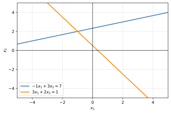
\[\begin{cases} -x_1 + 3x_2 = 7 \\ 3x_1 + 2x_2 = 1 \end{cases}\]
We separate the coefficient matrix \(A\) from the right-hand side vector \(b\):
A = np.array([[-1, 3],
              [3, 2]], dtype=float)

b = np.array([7, 1], dtype=float)

print("Matrix A:")
print(A)
print(f"\nVector b: {b}")
print(f"\nShape of A: {A.shape}")
print(f"Shape of b: {b.shape}")
Matrix A:
[[-1. 3.]
[ 3. 2.]]
Vector b: [7. 1.]
Shape of A: (2, 2)
Shape of b: (2,)We can also form the augmented matrix \([A | b]\) by stacking horizontally:
A_system = np.hstack((A, b.reshape(2, 1)))
print(A_system)
[[-1. 3. 7.]
[ 3. 2. 1.]]Solving and Verifying
d = np.linalg.det(A)
print(f"det(A) = {d:.2f}")

x = np.linalg.solve(A, b)
print(f"Solution: x1 = {x[0]:.0f}, x2 = {x[1]:.0f}")
det(A) = -11.00
Solution: x1 = -1, x2 = 2The determinant is nonzero (\(-11\)), so the system has exactly one solution. Let’s visualize — the two lines intersect at \((-1, 2)\):
No Solution (Parallel Lines)
Now consider:
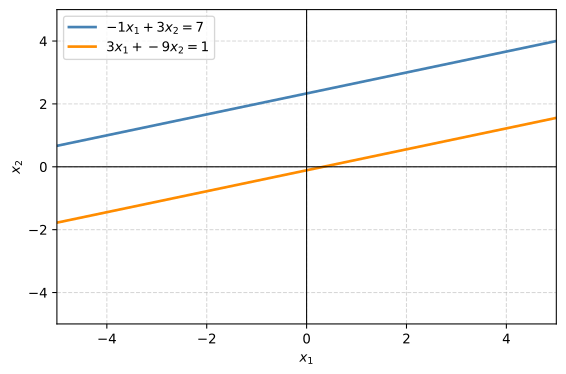
\[\begin{cases} -x_1 + 3x_2 = 7 \\ 3x_1 - 9x_2 = 1 \end{cases}\]
The second equation is \(-3\) times the first on the left side, but not on the right — a contradiction.
A_2 = np.array([[-1, 3],
                [3, -9]], dtype=float)
b_2 = np.array([7, 1], dtype=float)

print(f"det(A_2) = {np.linalg.det(A_2):.2f}")

try:
    np.linalg.solve(A_2, b_2)
except np.linalg.LinAlgError as e:
    print(f"Error: {e}")
det(A_2) = -0.00Determinant is zero and NumPy raises an error. The lines are parallel:
Infinitely Many Solutions (Same Line)
If we change the right-hand side so the equations are consistent:
\[\begin{cases} -x_1 + 3x_2 = 7 \\ 3x_1 - 9x_2 = -21 \end{cases}\]
Now the second equation is exactly \(-3\) times the first — same line, infinitely many solutions:
b_3 = np.array([7, -21], dtype=float)

A_3_system = np.hstack((A_2, b_3.reshape(2, 1)))
print("Augmented matrix:")
print(A_3_system)
print(f"\ndet = {np.linalg.det(A_2):.2f} (still singular)")
print("Solutions: x1 = 3*x2 - 7, where x2 is any real number")
Augmented matrix:
[[ -1. 3. 7.]
[ 3. -9. -21.]]
det = -0.00 (still singular)
Solutions: x1 = 3*x2 - 7, where x2 is any real number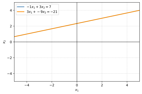
Both equations produce the same line — every point on it is a solution.
Summary
The determinant tells you everything about a \(2 \times 2\) system:
| Determinant | Lines | Solutions |
|---|---|---|
| \(\neq 0\) | Intersect at one point | Unique |
| \(= 0\) (contradictory) | Parallel | None |
| \(= 0\) (redundant) | Same line | Infinitely many |