Fine-tune DistilBERT for entity recognition on resumes and extractive question answering, and fix the label alignment bugs behind the original results.
Published
Aug 31, 2026
Building a Transformer Network implemented the architecture from scratch and ended with an untrained model of a few thousand parameters. This lab does the opposite. It starts from DistilBERT, a 66-million-parameter transformer that someone else already trained on a very large corpus, and adapts it to two tasks.
The lab merges the two ungraded application notebooks from the course, Named-Entity Recognition and Question Answering, because they are the same recipe applied twice. Load a pretrained body, attach a small task-specific head, tokenize the text with the tokenizer that model was trained with, align the labels to the subtokens the tokenizer produced, and train. The second task is told more briefly than the first, precisely because the recipe is already established.
The alignment step is where both notebooks go wrong, and this page spends real effort on it. Getting a label onto the right subtoken sounds like plumbing. It is not. Three separate defects in the original notebooks all live in that step, and together they are the difference between a model that appears to fail at eight of its twelve categories and one that works.
By the end of this lab you will be able to
turn character-offset entity annotations into per-subtoken labels without going through words, and see three ways the obvious word-based route loses or misplaces them,
explain why word_ids() from a fast tokenizer does not line up with text.split(), and what that costs,
fine-tune a pretrained transformer for token classification and for span extraction,
evaluate a heavily imbalanced classifier without fooling yourself with accuracy,
state which of a dataset’s defects actually limits a model and which merely looks like it should.
ImportantUpdated From the Original Assignments
The two source notebooks were written against TensorFlow 2.3, Keras 2, pandas 1.x and Hugging Face Transformers 4.5. This page runs on PyTorch 2.13, Transformers 5.15, NumPy 2.4 and scikit-learn 1.9 as installed in the project environment. Eleven things changed, on 2026-08-31.
Everything is PyTorch, because the TensorFlow classes no longer exist. Transformers 5 removed TensorFlow model support, so TFDistilBertForTokenClassification and TFDistilBertForQuestionAnswering are both gone and neither notebook runs as written. The PyTorch equivalents, DistilBertForTokenClassification and DistilBertForQuestionAnswering, load the same pretrained weights and are used throughout.
The duplicate implementations are collapsed into one. The question answering notebook implements the same model twice, once in TensorFlow with a tf.GradientTape loop and once in PyTorch with the Hugging Face Trainer. With TensorFlow gone, one implementation remains.
The Trainer is replaced with an explicit training loop.Trainer now requires the accelerate package, which is not in the project environment, and its progress output does not survive a static render. The loop below is a dozen lines and is deliberately plainer than what it replaces. Trainer would also apply a linear learning-rate schedule with warmup and exempt bias and normalization parameters from weight decay, and neither is reproduced here, so the run is a constant learning rate with AdamW applied uniformly. For question answering it computes the start-position and end-position cross-entropies separately and averages them, which is what the notebook’s own TensorFlow loop wrote as 0.5 * (loss_start + loss_end), and the page checks that it reproduces what the model computes internally when it is handed start_positions and end_positions.
Labels are attached to subtokens by character offset, not routed through words. The notebook’s clean_dataset builds a tag per whitespace-separated word and then copies it onto subtokens, and that intermediate step fails in three independent ways, each documented with its measured cost in “Three Ways to Lose or Misplace a Label” below. Runs of spaces cost 1,302 tags and an unflushed final word costs 7 more. Requiring a word to sit entirely inside an entity loses every word carrying attached punctuation, and loosening that to any overlap over-labels instead, taking a whole 97-character URL from a 44-character overlap. And the tokenizer’s notion of a word is not str.split()’s, so tags drift out of alignment from the first punctuation mark onward. Using return_offsets_mapping=True and comparing each subtoken’s character span against the annotation removes all three at once, in the coordinates the annotation was written in.
pandas is no longer used at all. The notebook’s tagging built a frame row by row with DataFrame.append, removed in pandas 2.0, and the project environment is on pandas 3.0.3. Offset-based labeling needs no frame, so the dependency is gone rather than ported.
Evaluation excludes the positions that carry no label. The notebook maps every label back through id2tag.get(index, "Empty"), which turns the -100 assigned to special tokens and padding into the Empty class. Reproducing its pipeline exactly gives the 103,155 positions it counts as Empty, of which 18,253 are special tokens and padding carrying no label at all. The other 84,902 are mapped to Empty rather than genuinely tagged, since 12,788 of them come from word indices that ran past the real tag array and read its padding. Either way, a large share of what it scores is not a measurement of the model. Positions labeled -100 are dropped here before any metric is computed.
seqeval is replaced by scikit-learn.seqeval scores IOB2 tagging, where labels look like B-Name and I-Name, and reads the first character as the chunk prefix and the rest as the entity type. These labels are plain, so it reported entity names of ame, kills, mpty, ocation and NKNOWN, each the label minus its first letter. That is the notebook’s own printed output, and it shows the metric was never measuring what it claimed. sklearn.metrics.classification_report scores the labels as they actually are, and is already a project dependency.
A train and test split is used. The notebook fits on all 220 resumes and then calls model.predict on the same 220, so every number it reports is a training-set number. An 80/20 split by document is used here, so the reported metrics are on 44 resumes the model never saw.
The optimizer is AdamW rather than Adam. The entity notebook used tf.keras.optimizers.Adam and the question answering notebook used Adam in its TensorFlow half and the Trainer defaults in its PyTorch half. AdamW applies decoupled weight decay, PyTorch’s default of 0.01, which the notebook’s TensorFlow paths did not. The learning rates are the notebook’s own. The Trainer half’s 20 warmup steps are not reproduced, since there is no scheduler here.
The entity model is given an attention mask. The notebook builds its dataset from input_ids and labels only, so the model attends over padding as though it were text. The mask the tokenizer already returns is passed here.
The question answering metric is exact match rather than macro F1 over positions. The notebook scores f1_score(start_labels, start_preds, average='macro'), which treats each token position as a class and averages over positions that mostly never occur. This page reports how often the predicted start, end, span and decoded answer text are exactly right, which is the standard measure for extractive question answering and is directly interpretable.
Left alone are both datasets, the pretrained checkpoint, the tokenizer, the task definitions, and the notebook’s epochs, learning rates and batch sizes, namely 10 epochs at \(10^{-5}\) with batches of 4 for the entity task and 3 epochs at \(3 \times 10^{-5}\) with batches of 8 for question answering. The optimizer and the evaluation are the exceptions, covered by items 9 and 11.
NoteLab Files Download
ner.json (1.2 MB), 220 resumes with character-offset entity annotations, in the format the Dataturks annotation tool exported.
The pretrained checkpoint is 253 MB, which is too large to host here. It is the distilbert-base-uncased body, available on the Hugging Face Hub, and from_pretrained("distilbert-base-uncased") fetches it.
The entity notebook ships only a TensorFlow tf_model.h5, which Transformers 5 cannot read. The question answering notebook ships both a TensorFlow and a PyTorch copy, and that PyTorch file is the checkpoint this page loads for both tasks. It is the distilbert-base-uncased body carrying an untrained question answering head, saved before anyone fine-tuned it. That detail matters for reproducing the loading reports below. The Hub’s distilbert-base-uncased carries a masked-language-model head instead, so loading it for question answering reports qa_outputs as newly initialized where the course checkpoint reports nothing missing. The trained body, which is what actually matters, is identical either way.
DistilBERT is the distilled model of Sanh et al. (2019), a smaller and faster version of BERT, the model of Devlin et al. (2018), that keeps most of its accuracy. It has 6 layers rather than 12 and 66 million parameters rather than 110 million, which is what makes it practical to fine-tune twice inside a page render. Both are encoder-only, so they reuse the self-attention, position-wise feed-forward, residual and layer-normalization pieces the previous lab built for the encoder, and none of its decoder. They also learn their position embeddings as ordinary parameters rather than fixing them to the sine and cosine curves of Vaswani et al. (2017).
import jsonimport reimport timeimport numpy as npimport torchimport matplotlib.pyplot as pltfrom collections import Counterimport datasetsimport transformersfrom datasets import load_from_diskfrom sklearn.metrics import classification_report, accuracy_scorefrom transformers import (DistilBertTokenizerFast, DistilBertForTokenClassification, DistilBertForQuestionAnswering)MEDIA ="../../../media/deep-learning/fine-tuning-a-pretrained-transformer/"# Progress bars render as empty widget placeholders in a static page.datasets.disable_progress_bars()# map() otherwise writes cache files next to the dataset, inside media/.datasets.disable_caching()transformers.utils.logging.disable_progress_bar()transformers.utils.logging.set_verbosity_error()# Apple silicon exposes its GPU as "mps", CUDA machines as "cuda". Either is# substantially faster than the CPU for this, though the exact factor depends# on the machine. The page runs correctly on any of the three.device = torch.device("mps"if torch.backends.mps.is_available()else"cuda"if torch.cuda.is_available()else"cpu")print("PyTorch", torch.__version__, "| device:", device)
PyTorch 2.13.0 | device: mps
The tokenizer is loaded once and used for both tasks, because both tasks use the same model. This is not optional. A tokenizer defines the integer that each piece of text maps to, and a pretrained model’s weights are only meaningful against the exact vocabulary it was trained with.
is_fast being true is what makes the rest of this lab possible. The fast tokenizers are backed by the Rust tokenizers library and are the only ones that can report where each subtoken came from. The entity task uses return_offsets_mapping=True to get each subtoken’s character span, and the question answering task uses char_to_token() to go the other way, from a character offset to the subtoken holding it. Both alignment steps depend on exactly that.
Named-Entity Recognition on Resumes
Named-entity recognition finds the pieces of a text that name something and says what kind of thing each one names. In the sentence “Jane visits Africa in September”, the entities are Jane as a person, Africa as a location and September as a time.
The dataset here is 220 resumes, each annotated with spans marking names, designations, companies, colleges, degrees, skills and a few other categories. A working model of this kind is what sits behind a system that reads a stack of applications and fills in a form.
Reading the Annotations
Each line of ner.json is one resume. The content field holds the raw text and annotation holds a list of spans, each with a label and a character offset into that text.
The loader does three small jobs. It replaces newlines with spaces so the text is one line, it converts each annotation’s inclusive end offset into the exclusive end that Python slicing expects, and it trims whitespace off both ends of every span, since the annotators frequently included the trailing newline in the highlighted text.
def load_resumes(path):"""Read the annotation file into (text, [(start, end, label), ...]) pairs.""" documents = []for line inopen(path): record = json.loads(line) text = record['content'].replace("\n", " ") spans = []for annotation in (record['annotation'] or []): point = annotation['points'][0] labels = annotation['label']ifnotisinstance(labels, list): labels = [labels]for label in labels:# The file's 'end' is inclusive, so add one for a Python slice. start, end = point['start'], point['end'] +1# Annotators often selected leading or trailing whitespace.# Pull both ends in until they sit on real characters. highlighted = point['text'] start +=len(highlighted) -len(highlighted.lstrip()) end -=len(highlighted) -len(highlighted.rstrip())while start <len(text) and text[start].isspace(): start +=1while end >1and text[end -1].isspace(): end -=1 spans.append((start, end, label)) documents.append((text, spans))return documentsdocuments = load_resumes(MEDIA +"ner.json")print("documents:", len(documents))print("annotated spans:", sum(len(s) for _, s in documents))
documents: 220
annotated spans: 3556
One document’s first few spans show what the offsets refer to. Slicing the text with them should recover exactly the entity text.
first 90 characters: 'Abhishek Jha Application Development Associate - Accenture  Bengaluru, Karnataka - Email m'

  [   0,   12)  Name                   -> 'Abhishek Jha'
  [  13,   46)  Designation            -> 'Application Development Associate'
  [  49,   58)  Companies worked at    -> 'Accenture'
  [  60,   69)  Location               -> 'Bengaluru'
  [  95,  145)  Email Address          -> 'Indeed: indeed.com/r/Abhishek-Jha/10e7a8cb732bc43a'
Labeling Subtokens Directly
The annotations give character offsets. The model consumes subtokens. Getting from one to the other is the whole of the preparation, and it is where all three of the original’s defects live.
The natural-looking route is to go through words. Tag each word, then copy each word’s tag onto the subtokens it produced. That is what the notebook does, and it is where it goes wrong, because “word” means three different things to the three pieces of code involved.
WarningThree Ways to Lose or Misplace a Label
Every one of these is silent. None raises, and each leaves the shapes intact.
Runs of spaces. The notebook walks the text one character at a time and assigns a tag whenever it reaches a space, testing that space’s index against the end of the entity. Where a word is followed by more than one space, the test fires on the last space of the run, whose index is past the end of the span, and the tag is dropped. The loader turns every newline into a space, so a line break followed by an indent becomes a run of spaces, and there are 6,965 such runs across the 220 documents. Accenture in the first resume is a casualty. It occupies characters 49 to 58 and is followed by two spaces, so the original tests 59 <= 58, which is false, and the entity’s only word goes untagged. This costs 1,302 tags, and a further 7 are lost because the loop never flushes the final word of a document.
Word boundaries that do not match annotation boundaries. The test also demands that a word sit entirely inside the span. Annotators marked Bengaluru as a Location, characters 60 to 69, but the text reads Bengaluru, and whitespace splitting keeps the comma attached, giving a word spanning 60 to 70. A containment test asks 70 <= 69 and fails, so the word is tagged Empty. Loosening it to accept any overlap is not a fix either, because it then labels the whole of a 97-character URL from a 44-character overlap. Neither answer is right, because the question is wrong. The word is the wrong unit.
word_ids() does not count words the way split() does. The notebook builds its tags from text.split(), which splits on whitespace only, and then indexes them with word_ids(), which reports the tokenizer’s own pre-tokenizer, which splits on whitespace and punctuation. From the first punctuation mark in a document onward, the two indices drift apart and every tag lands on the wrong word. Within the notebook’s 512-subtoken truncation the tokenizer reports more words than split() in 118 of the 220 documents, and without truncation the two disagree in all 220. It raises no error because the tag array was padded to 512 before the lookup, so an index that has run off the end still finds an entry, which holds padding.
The fix is to stop going through words. A fast tokenizer will report the character span each subtoken came from, so a subtoken can be compared against the annotation directly, in the coordinates the annotation was written in. Every one of the three problems above is a property of the intermediate word step, and none of them survives its removal.
return_offsets_mapping=True asks the tokenizer for those spans. Each subtoken comes back with the half-open character range it covers, and special tokens and padding come back as (0, 0), which is how they are recognized. A subtoken is labeled with an entity if the two ranges overlap at all, taking the same reverse-order precedence the original used, so a span listed later in the file wins.
MAX_LEN =512unique_tags =sorted({label for _, spans in documents for*_, label in spans} | {"Empty"})tag2id = {tag: i for i, tag inenumerate(unique_tags)}id2tag = {i: tag for tag, i in tag2id.items()}def encode(documents):"""Label every subtoken by comparing its character span to the annotations.""" encoded = tokenizer([text for text, _ in documents], truncation=True, padding='max_length', max_length=MAX_LEN, return_offsets_mapping=True) labels = []for i, (_, spans) inenumerate(documents): row = []for start, end in encoded['offset_mapping'][i]:if start == end:# A special token or padding. -100 tells the loss to skip it. row.append(-100)continue tag ="Empty"for span_start, span_end, label inreversed(spans):if start < span_end and end > span_start: tag = labelbreak row.append(tag2id[tag]) labels.append(row) encoded['labels'] = labelsreturn encodedencoded = encode(documents)input_ids = np.array(encoded['input_ids'])attention_mask = np.array(encoded['attention_mask'])labels = np.array(encoded['labels'])print("tags:", len(unique_tags))print("input_ids:", input_ids.shape, "| labels:", labels.shape)
Reading the alignment back out is the check that it worked, and the interesting rows are the ones the word-based route got wrong.
subtokens = tokenizer.convert_ids_to_tokens(input_ids[0])offsets = encoded['offset_mapping'][0]text = documents[0][0]print(f"{'subtoken':14}{'offsets':>12}{'text there':14} tag")for j inrange(0, 18): start, end = offsets[j] covered =repr(text[start:end]) if end > start else"(special)" tag = id2tag[labels[0][j]] if labels[0][j] !=-100else"-100, ignored"print(f"{subtokens[j]!r:14}{str(tuple(offsets[j])):>12}{covered:14}{tag}")
subtoken            offsets  text there     tag
'[CLS]'              (0, 0)  (special)      -100, ignored
'ab'                 (0, 2)  'Ab'           Name
'##his'              (2, 5)  'his'          Name
'##he'               (5, 7)  'he'           Name
'##k'                (7, 8)  'k'            Name
'j'                 (9, 10)  'J'            Name
'##ha'             (10, 12)  'ha'           Name
'application'      (13, 24)  'Application'  Designation
'development'      (25, 36)  'Development'  Designation
'associate'        (37, 46)  'Associate'    Designation
'-'                (47, 48)  '-'            Empty
'accent'           (49, 55)  'Accent'       Companies worked at
'##ure'            (55, 58)  'ure'          Companies worked at
'bengal'           (60, 66)  'Bengal'       Location
'##uru'            (66, 69)  'uru'          Location
','                (69, 70)  ','            Empty
'karnataka'        (71, 80)  'Karnataka'    Empty
'-'                (81, 82)  '-'            Empty
Both subtokens of Accenture carry Companies worked at, which the original dropped to the space run. bengal and ##uru carry Location, which containment dropped. And the comma, whose offsets are (69, 70) against a Location span ending at 69, correctly carries Empty, which any-overlap on whole words would have got wrong. None of that needed a rule about punctuation. It falls out of comparing character ranges.
The number of positions that actually carry a label is worth knowing before any metric is computed.
real = labels !=-100print(f"positions carrying a label: {real.sum():,} of {labels.size:,} "f"({100* real.sum() / labels.size:.1f}%)")print()for tag, count in Counter(id2tag[i] for i in labels[real]).most_common():print(f" {tag:22}{count:7,}")
positions carrying a label: 94,387 of 112,640 (83.8%)

  Empty                   76,777
  Email Address            5,951
  Skills                   5,113
  Designation              1,439
  Companies worked at      1,216
  Name                     1,056
  College Name             1,051
  Location                   772
  Degree                     756
  Graduation Year            146
  Years of Experience        110
Note how heavily subword splitting reweights the categories. Email Address is a small number of words but nearly 6,000 subtokens, because an address such as indeed.com/r/Abhishek-Jha/10e7a8cb732bc43a fragments into a couple of dozen pieces. Subtoken counts, not word counts, are what the loss actually sees, and a category made of long unusual strings therefore carries far more weight per occurrence than its word count suggests.
Fine-Tuning
Loading the checkpoint with num_labels=12 gives DistilBERT’s pretrained body with a fresh linear classifier on top. Transformers reports exactly which weights came from the file and which were created new, and reading that report is a habit worth forming, because it is where a silently mismatched checkpoint announces itself.
The split is by document, so no resume contributes to both training and evaluation.
Now the model itself. Passing output_loading_info=True makes from_pretrained return the report alongside the model instead of only logging it.
torch.manual_seed(0)ner_model, loading_info = DistilBertForTokenClassification.from_pretrained( MEDIA +"distilbert-base-uncased", num_labels=len(unique_tags), output_loading_info=True)ner_model = ner_model.to(device)print("parameters:", sum(p.numel() for p in ner_model.parameters()))print("newly initialized:", sorted(loading_info['missing_keys']))print("in the file but unused:", sorted(loading_info['unexpected_keys']))
parameters: 66372108
newly initialized: ['classifier.bias', 'classifier.weight']
in the file but unused: ['qa_outputs.bias', 'qa_outputs.weight']
Read that report every time. from_pretrained loads what it recognizes, randomly initializes what it cannot find, and drops what it does not need, all without raising, so this is the only place a wrong checkpoint announces itself.
Here it says the right thing. The two classifier tensors are the fresh linear head, and they are the only randomly initialized parameters in the model. The two qa_outputs tensors are a question answering head the file carries and this task has no use for. Every weight in the six transformer layers loaded from the file, which is the knowledge that makes 176 resumes enough.
The training loop is the standard PyTorch four lines. Forward, backward, step, zero. Passing labels to the model makes it compute the cross-entropy itself, skipping every position labeled -100.
optimizer = torch.optim.AdamW(ner_model.parameters(), lr=1e-5)start_time = time.time()ner_losses = []for epoch inrange(10): ner_model.train() total =0.0for ids, mask, label_batch in train_loader: output = ner_model(input_ids=ids.to(device), attention_mask=mask.to(device), labels=label_batch.to(device)) output.loss.backward() optimizer.step() optimizer.zero_grad() total += output.loss.item() ner_losses.append(total /len(train_loader))print(f"epoch {epoch +1:2} train loss {ner_losses[-1]:.4f}"f" [{time.time() - start_time:.0f}s]")
epoch  1  train loss 1.1398  [7s]
epoch  2  train loss 0.6923  [15s]
epoch  3  train loss 0.5135  [22s]
epoch  4  train loss 0.4033  [29s]
epoch  5  train loss 0.3232  [36s]
epoch  6  train loss 0.2844  [44s]
epoch  7  train loss 0.2482  [51s]
epoch  8  train loss 0.2144  [58s]
epoch  9  train loss 0.1798  [65s]
epoch 10  train loss 0.1588  [72s]
Evaluating Without Fooling Yourself
Predictions are collected over the held-out resumes, keeping only the positions that carry a real label.
Accuracy alone would have been close to worthless here. A model that answered Empty at every position and nothing else would score the baseline above, and the gap between that and the real number is the only part of the accuracy figure that carries information. The per-class report is where the model is actually judged.
                     precision    recall  f1-score   support

       College Name      0.750     0.695     0.722       246
Companies worked at      0.541     0.512     0.526       258
             Degree      0.758     0.706     0.731       204
        Designation      0.710     0.705     0.707       288
      Email Address      0.792     0.829     0.810      1041
              Empty      0.953     0.944     0.948     15043
    Graduation Year      0.000     0.000     0.000        32
           Location      0.731     0.449     0.556       236
               Name      0.923     0.949     0.936       215
             Skills      0.521     0.764     0.620       622
            UNKNOWN      0.000     0.000     0.000         0
Years of Experience      0.000     0.000     0.000        27

           accuracy                          0.906     18212
          macro avg      0.557     0.546     0.546     18212
       weighted avg      0.908     0.906     0.906     18212
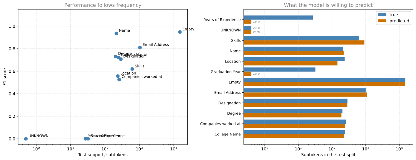
Read the support column against the f1-score column and the floor is unmistakable. The categories the model handles well are the ones it saw most often, and the three it scores zero on are the three with the least to go on, two of them with a few dozen held-out subtokens and one with none at all.
UNKNOWN is a special case worth reading carefully, because its zero support is not simple bad luck in the split. The label is annotated in two documents only, and one of them is in the test set. Its occurrence there sits past word 375 of a 471-word resume, well beyond the point where 512 subtokens run out, so truncation removed it before the model or the metric ever saw it. Truncation is a quiet way to lose exactly the rare material that long documents carry, and a category whose support is zero is always worth tracing back rather than assuming it was never sampled.
%config InlineBackend.figure_formats = ['svg']report = classification_report(gold, predicted, labels=list(range(len(unique_tags))), target_names=unique_tags, zero_division=0, output_dict=True)support = np.array([report[t]['support'] for t in unique_tags])f1 = np.array([report[t]['f1-score'] for t in unique_tags])true_counts = np.array([(gold == i).sum() for i inrange(len(unique_tags))])pred_counts = np.array([(predicted == i).sum() for i inrange(len(unique_tags))])fig, axes = plt.subplots(1, 2, figsize=(14, 5.5))axes[0].scatter(np.maximum(support, 0.5), f1, s=60, color='#4682B4', zorder=3)for tag, x, y inzip(unique_tags, np.maximum(support, 0.5), f1): axes[0].annotate(tag, (x, y), fontsize=9, xytext=(6, 4), textcoords='offset points')axes[0].set_xscale('log')axes[0].set_xlabel('Test support, subtokens')axes[0].set_ylabel('F1 score')axes[0].set_ylim(-0.05, 1.15)axes[0].grid(linestyle='--', alpha=0.4)axes[0].set_title('Performance follows frequency', fontsize=12, color='gray')y = np.arange(len(unique_tags))# A log axis cannot show a zero, so zero counts are drawn as a visible stub# at 0.4 and marked, rather than vanishing without explanation.axes[1].barh(y +0.2, np.maximum(true_counts, 0.4), height=0.4, color='#4682B4', label='true')axes[1].barh(y -0.2, np.maximum(pred_counts, 0.4), height=0.4, color='#CC7000', label='predicted')for yi, (t, p) inenumerate(zip(true_counts, pred_counts)):for offset, count in ((0.2, t), (-0.2, p)):if count ==0: axes[1].text(0.45, yi + offset, 'zero', va='center', fontsize=7.5, color='#727B86')axes[1].set_xscale('log')axes[1].set_yticks(y)axes[1].set_yticklabels(unique_tags, fontsize=9)axes[1].set_xlabel('Subtokens in the test split')axes[1].legend()axes[1].grid(axis='x', linestyle='--', alpha=0.4)axes[1].set_title('What the model is willing to predict', fontsize=12, color='gray')plt.tight_layout()plt.show()
On the left, how many held-out subtokens each category has against the F1 the model achieves on it, with support on a logarithmic axis. The relationship is loose rather than monotone, since several categories with a few hundred subtokens differ widely, but the floor is clear. Nothing below about a hundred held-out subtokens gets off zero, and nothing above a thousand does badly. On the right, the number of subtokens the model assigns to each category against the true number, with zero counts drawn as labeled stubs because a logarithmic axis cannot show them. The frequent categories are produced at roughly the right rate, while the categories scoring zero are never emitted at all, which is what a zero F1 means in practice here. The model is not confused about those. It has decided they do not exist.
The honest summary of this model is that it reads a resume’s name and email address well, handles degrees, colleges, job titles and locations reasonably, gets companies and skills right around half to two-thirds of the time, and is blind to graduation years and years of experience. That is a far more useful thing to know than a single accuracy number, and it points directly at what to do next, which is to get more examples of the rare categories rather than to train longer.
It is also worth remembering how close this model came to being blind to locations too. Routing labels through whitespace words, in either the containment or the any-overlap form, mangles most Location annotations, and the report then shows a zero that looks exactly like a rare category the model failed to learn. A category scoring zero is a prompt to check the labels before concluding anything about the model.
Extractive Question Answering
The second task changes almost nothing about the method. Load the same pretrained body, attach a different head, align labels to subtokens, train. What changes is what the head predicts. Instead of a class per token, it predicts two positions, where the answer starts and where it ends.
That is what extractive means. The model does not compose an answer, it points at one. Asked “When will Jane go to Africa?” over the text “Jane visits Africa in September”, it returns the span covering September rather than generating the word.
bAbI Dataset
The data is the bAbI question answering set of Weston et al. (2015), a collection of deliberately simple synthetic stories built to isolate individual reasoning skills. Each story here is two statements about where rooms are relative to each other and one question.
DatasetDict({
    train: Dataset({
        features: ['story'],
        num_rows: 1000
    })
    test: Dataset({
        features: ['story'],
        num_rows: 1000
    })
})

{'answer': ['', '', 'office'], 'id': ['1', '2', '3'], 'supporting_ids': [[], [], ['1']], 'text': ['The office is north of the kitchen.', 'The garden is south of the kitchen.', 'What is north of the kitchen?'], 'type': [0, 0, 1]}
Each of the three entries carries an id, a type of 0 for a statement and 1 for a question, an answer that is empty for the statements, and a list of supporting ids naming which statements are needed to answer. Every story in both splits has the same [0, 0, 1] shape, so the structure can be relied on.
Flattening turns the nested dictionary into columns, and two small mapped functions pull out the three fields the task needs.
context:  The hallway is south of the garden. The garden is south of the bedroom.
question: What is south of the bedroom?
answer:   garden
Locating the Answer in the Text
The label is not the answer word, it is where the answer word sits. find returns the character offset of the first occurrence, and the end follows from the answer’s length.
That example is worth pausing on. The context reads “The hallway is south of the garden. The garden is south of the bedroom.” and the question is “What is south of the bedroom?”. The word garden appears twice, and find points at the first one, in the sentence about the hallway. The dataset’s own supporting_ids names the second sentence as the one that answers the question. The label therefore points at the wrong occurrence of the right word.
def count_ambiguous(split): multiple = disagreeing =0for row in babi.flatten()[split]: first_sentence, second_sentence, _ = row['story.text'] answer = row['story.answer'][2] context = first_sentence +' '+ second_sentence supporting = row['story.supporting_ids'][2][0] target, offset = ((first_sentence, 0) if supporting =='1'else (second_sentence, len(first_sentence) +1))if context.count(answer) >1: multiple +=1if context.find(answer) != offset + target.find(answer): disagreeing +=1return multiple, disagreeingfor split in ('train', 'test'): multiple, disagreeing = count_ambiguous(split)print(f"{split}: answer appears more than once in {multiple}/1000 stories, "f"and find() disagrees with the supporting fact in {disagreeing}/1000")
train: answer appears more than once in 345/1000 stories, and find() disagrees with the supporting fact in 167/1000
test: answer appears more than once in 343/1000 stories, and find() disagrees with the supporting fact in 158/1000
So about a third of the stories contain their answer word twice, and in about a sixth of them the label points somewhere the dataset does not consider the source of the answer. “Does the Labeling Ambiguity Matter?” below tests whether that is worth fixing, which turns out to have a more interesting answer than it looks.
Aligning Positions to Subtokens
The same alignment problem returns in a different shape. The offsets are into characters, and the model indexes subtokens, so the two have to be connected. char_to_token is the fast tokenizer’s method for exactly that.
The context and the question are tokenized together as a pair, so the model sees [CLS] context [SEP] question [SEP] and answers by pointing into it. Note the order. Hugging Face’s own question answering examples put the question first, and this lab puts the context first. Either works, because the model learns whichever arrangement it is fine-tuned on, but the two are not interchangeable at inference and the order used in training has to be the order used afterward.
def tokenize_align(example):"""Encode the context and question together, and convert the answer's character offsets into subtoken positions.""" encoded = tokenizer(example['sentences'], example['question'], truncation=True, max_length=tokenizer.model_max_length) start_position = encoded.char_to_token(example['str_idx'])# end_idx is exclusive, so ask about the last character of the answer. end_position = encoded.char_to_token(example['end_idx'] -1)# A None means the offset landed in a gap, such as a space, or outside the# truncated span. Mark those -100 so the loss skips them. The notebook# instead pointed them at model_max_length, which is a valid target only# because the model it used clamped out-of-range positions internally.return {'input_ids': encoded['input_ids'],'attention_mask': encoded['attention_mask'],'start_positions': -100if start_position isNoneelse start_position,'end_positions': -100if end_position isNoneelse end_position}qa_dataset = processed.map(tokenize_align)row = qa_dataset['train'][200]tokens = tokenizer.convert_ids_to_tokens(row['input_ids'])print("context: ", row['sentences'])print("question:", row['question'])print("answer: ", row['answer'])print(f"positions {row['start_positions']} to {row['end_positions']}"f" -> {tokens[row['start_positions']:row['end_positions'] +1]}")print()print("tokens:", tokens)
context:  The garden is north of the bathroom. The hallway is south of the bathroom.
question: What is north of the bathroom?
answer:   garden
positions 2 to 2 -> ['garden']

tokens: ['[CLS]', 'the', 'garden', 'is', 'north', 'of', 'the', 'bathroom', '.', 'the', 'hallway', 'is', 'south', 'of', 'the', 'bathroom', '.', '[SEP]', 'what', 'is', 'north', 'of', 'the', 'bathroom', '?', '[SEP]']
Every story in this dataset produces exactly 26 subtokens, because the sentences are generated from a small set of templates. That is unusual and convenient, since it means no padding is needed and the attention mask is all ones.
lengths = {len(row) for row in qa_dataset['train']['input_ids']}print("distinct sequence lengths in the training split:", lengths)print("start positions range from",min(qa_dataset['train']['start_positions']), "to",max(qa_dataset['train']['start_positions']))print("stories with no locatable answer:",sum(p ==-100for split in ('train', 'test')for p in qa_dataset[split]['start_positions']))
distinct sequence lengths in the training split: {26}
start positions range from 2 to 10
stories with no locatable answer: 0
Fine-Tuning
The model is DistilBertForQuestionAnswering, the same body with a head that produces two numbers per position, a start score and an end score. Given start_positions and end_positions it computes a cross-entropy on each and averages them, so one loss covers both.
def make_qa_dataset(split): rows = qa_dataset[split] width =max(len(r) for r in rows['input_ids']) ids = torch.zeros(len(rows), width, dtype=torch.long) mask = torch.zeros(len(rows), width, dtype=torch.long)for i, (row_ids, row_mask) inenumerate(zip(rows['input_ids'], rows['attention_mask'])): ids[i, :len(row_ids)] = torch.tensor(row_ids) mask[i, :len(row_mask)] = torch.tensor(row_mask)return torch.utils.data.TensorDataset(ids, mask, torch.tensor(rows['start_positions']), torch.tensor(rows['end_positions']))qa_train = torch.utils.data.DataLoader(make_qa_dataset('train'), batch_size=8, shuffle=True)qa_test = torch.utils.data.DataLoader(make_qa_dataset('test'), batch_size=8)print(f"train {len(qa_dataset['train'])} stories, test {len(qa_dataset['test'])} stories")
train 1000 stories, test 1000 stories
The same checkpoint loads differently for this head, which is worth seeing next to the report from the entity task.
_, qa_loading_info = DistilBertForQuestionAnswering.from_pretrained( MEDIA +"distilbert-base-uncased", output_loading_info=True)print("newly initialized:", sorted(qa_loading_info['missing_keys']) or"nothing")print("in the file but unused:", sorted(qa_loading_info['unexpected_keys']) or"nothing")
newly initialized: nothing
in the file but unused: nothing
Nothing is missing and nothing is spare, because the checkpoint was saved as a question answering model and this is a question answering model. The qa_outputs head that the token classifier discarded is the one being loaded here. It is still untrained, since the checkpoint was saved before anyone fine-tuned it, which is why the loss below starts high rather than low.
def train_qa(train_loader, epochs=3, lr=3e-5, seed=0):"""Fine-tune a fresh question answering head and return the model and losses.""" torch.manual_seed(seed) model = DistilBertForQuestionAnswering.from_pretrained( MEDIA +"distilbert-base-uncased").to(device) optimizer = torch.optim.AdamW(model.parameters(), lr=lr) step_losses = []for epoch inrange(epochs): model.train() totals = np.zeros(3)for ids, mask, starts, ends in train_loader: output = model(input_ids=ids.to(device), attention_mask=mask.to(device))# Two independent classification problems over token positions.# cross_entropy skips targets of -100 by default, which is how the# stories with no locatable answer are excluded. start_loss = torch.nn.functional.cross_entropy(output.start_logits, starts.to(device)) end_loss = torch.nn.functional.cross_entropy(output.end_logits, ends.to(device)) loss =0.5* (start_loss + end_loss) loss.backward() optimizer.step() optimizer.zero_grad() step_losses.append(loss.item()) totals += [start_loss.item(), end_loss.item(), loss.item()] start_mean, end_mean, mean = totals /len(train_loader)print(f"epoch {epoch +1} start {start_mean:.4f} end {end_mean:.4f} mean {mean:.4f}")return model, step_lossesqa_model, qa_losses = train_qa(qa_train)
epoch 1  start 0.8477  end 0.8445  mean 0.8461
epoch 2  start 0.4223  end 0.4207  mean 0.4215
epoch 3  start 0.3263  end 0.3258  mean 0.3261
The averaging is not a choice this page invented. Handing start_positions and end_positions straight to the model produces the same number, which is worth confirming once rather than asserting. The two agree because every story here has a locatable answer. They would not agree on a -100, since cross_entropy skips that target while the model clamps out-of-range positions instead of ignoring them.
explicit 0.5 * (start + end): 0.159865
the model's own output.loss:  0.159865
difference: 0.00e+00
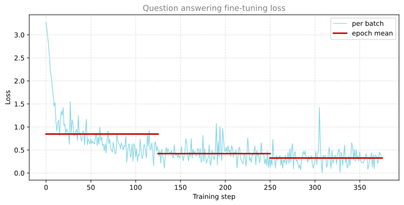
The start and end losses stay close to each other throughout, which is what you would expect when the answer is usually a single token and the two heads are solving nearly the same problem. Plotting every batch rather than the epoch means shows how much of that average is noise.
Loss on every one of the 375 training batches, with the per-epoch mean drawn over it. The fall is steep in the first epoch and then flattens, which is the usual shape for fine-tuning, because the body already knows the language and only the head and the last few layers need to move. The scatter within an epoch stays wide throughout, since a batch of 8 short stories is a noisy estimate of the gradient.
Results
Two things are worth measuring. Whether the model points at the exact positions the label names, and whether the text it returns is the right answer. Those are not the same question, and the difference between them is what the ambiguity above is about.
def evaluate_qa(model, loader, split='test'):"""Score exact position matches and exact answer text matches.""" model.eval() start_hits = end_hits = span_hits = text_hits = total =0 answers = [a.lower() for a in qa_dataset[split]['answer']] row =0with torch.no_grad():for ids, mask, starts, ends in loader: output = model(input_ids=ids.to(device), attention_mask=mask.to(device)) pred_start = output.start_logits.argmax(-1).cpu() pred_end = output.end_logits.argmax(-1).cpu() start_hits += (pred_start == starts).sum().item() end_hits += (pred_end == ends).sum().item() span_hits += ((pred_start == starts) & (pred_end == ends)).sum().item()for k inrange(len(starts)): tokens = tokenizer.convert_ids_to_tokens(ids[k]) answer =' '.join(tokens[pred_start[k]:pred_end[k] +1]).replace(' ##', '') text_hits += answer == answers[row] row +=1 total +=len(starts)return {'start': start_hits / total, 'end': end_hits / total,'span': span_hits / total, 'text': text_hits / total}scores = evaluate_qa(qa_model, qa_test)print(f"start position correct: {scores['start']:.4f}")print(f"end position correct: {scores['end']:.4f}")print(f"both correct: {scores['span']:.4f}")print(f"answer text correct: {scores['text']:.4f}")
start position correct: 0.7630
end position correct:   0.7600
both correct:           0.7580
answer text correct:    0.7580
The last two numbers being identical is the informative part. Whenever the model gets the span wrong, it also gets the text wrong. It never quietly picks the other occurrence of the right word and gets the answer right by a different route, which is what you would see if the ambiguity were driving the errors.
Does the Labeling Ambiguity Matter?
The measurement above found that find labels the wrong occurrence in about a sixth of the stories. That looks like a ceiling on performance, and the obvious next move is to fix it by using the supporting fact the dataset already provides and seeing the score rise.
def get_start_end_idx_supported(story):"""Locate the answer inside the sentence the dataset names as the supporting fact, rather than simply taking the first occurrence.""" supporting = story['story.supporting_ids'][2][0] first_sentence, second_sentence = story['story.text'][0], story['story.text'][1] target, offset = ((first_sentence, 0) if supporting =='1'else (second_sentence, len(first_sentence) +1)) start = offset + target.find(story['answer'])return {'str_idx': start, 'end_idx': start +len(story['answer'])}supported = (babi.flatten() .map(get_question_and_facts) .map(get_start_end_idx_supported) .map(tokenize_align))changed =sum(a != b for a, b inzip(qa_dataset['train']['start_positions'], supported['train']['start_positions']))print(f"training labels that moved: {changed} of 1000")
training labels that moved: 167 of 1000
That is the 167 stories counted earlier. Training a fresh model on the corrected labels and scoring it the same way gives a like-for-like comparison, since only the labels differ.
epoch 1  start 0.8558  end 0.8536  mean 0.8547
epoch 2  start 0.5784  end 0.5792  mean 0.5788
epoch 3  start 0.3065  end 0.3092  mean 0.3078

                          find()   supporting fact
  start correct           0.7630            0.7810  (own gold set)
  end correct             0.7600            0.7760  (own gold set)
  span correct            0.7580            0.7630  (own gold set)
  text correct            0.7580            0.7630  <- comparable
Only the last row compares like with like. Each model is scored against the labels it was trained on, so the two position columns are measured against different gold sets and a difference between them could just as well be a difference between the two definitions of where the answer is. The decoded answer text has no such problem, because both conditions share the same answer strings and the metric does not care which occurrence of the word was pointed at.
On the comparable row the two differ by under a point, and which of them comes out ahead is not stable. Both models are trained from the same seed, but fine-tuning on a GPU accumulates in a nondeterministic order, so re-rendering this page moves each figure by a few tenths of a point and has put the corrected-label column on both sides of the original. A single pair of runs cannot resolve a difference that small. Settling it would need several seeds in each condition and a paired comparison on the same test items, which this page does not do.
What can be said is bounded and still worth saying. Set the observed difference against what the defect allowed for. The wrong occurrence was named in 15.8 percent of the test labels. Note that this was never 15.8 points of available exact-match gain, since a model pointing at the other occurrence of the right word already scores as correct on text. What it was is 15.8 percent of the training signal pointing somewhere the dataset itself does not consider the source of the answer, which is the kind of noise that should degrade what the model learns. It moved the comparable score by a fraction of a point in an unstable direction. Whatever the remaining quarter of the errors are, this is not it.
That is worth sitting with, because the reasoning that led to the fix was sound and the payoff was still nothing. A defect being present in the data does not make it the thing holding a model back, and the only way to find out what is would be to look at the failures rather than to keep correcting the defects that are easy to see.
Asking a Question
The trained model, driven the way a user would drive it, with a question and a passage as plain strings. The first two stories are held out and the third is one the model trained on.
def answer_question(model, question, context): encoded = tokenizer(context, question, return_tensors='pt')with torch.no_grad(): output = model(**{k: v.to(device) for k, v in encoded.items()}) tokens = tokenizer.convert_ids_to_tokens(encoded['input_ids'][0]) start = output.start_logits.argmax(-1)[0] end = output.end_logits.argmax(-1)[0]return' '.join(tokens[start:end +1]).replace(' ##', '').capitalize()questions = [ ('What is south of the bedroom?','The hallway is south of the garden. The garden is south of the bedroom.'), ('What is east of the hallway?','The kitchen is east of the hallway. The garden is south of the bedroom.'), ('What is north of the kitchen?','The office is north of the kitchen. The garden is south of the kitchen.'),]for question, context in questions:print(f"{question:32}{answer_question(qa_model, question, context)}")
What is south of the bedroom?    Garden
What is east of the hallway?     Kitchen
What is north of the kitchen?    Office
NoteWhat You Should Remember
Fine-tuning is one recipe applied to different heads. The body is the same 66 million pretrained parameters in both halves of this lab, and only the layer on top and the loss change.
A pretrained model must be fed by its own tokenizer. The weights are meaningful only against the vocabulary they were trained with.
Subword tokenizers break the correspondence between words and model inputs. Do not route labels through words to repair it. Ask a fast tokenizer for return_offsets_mapping=True and compare each subtoken’s character span against the annotation, in the coordinates the annotation was written in.
Label -100 on special tokens and padding so the loss skips them, and drop those positions again before computing any metric. Folding them into a real class turns the metric into a measurement of padding.
Accuracy on an imbalanced problem is close to meaningless on its own. Quote the majority-class baseline next to it, and read the per-class report to find out what the model actually does.
A model can score zero on a class by never predicting it, which is a different failure from confusing it with another class and calls for different action.
Evaluate on data the model has not trained on. The original notebook fit and predicted on the same 220 resumes.
A defect you can find in the data is not automatically the reason a model underperforms. The ambiguous answer labels here were real and affected a sixth of the test set, and correcting them changed the score by less than the run-to-run noise. A category scoring zero, on the other hand, was a labeling bug, and that one was worth every minute.
Review Questions
1. Every subtoken inside an entity gets that entity’s label. Does that double-count long entities against short ones?
Answer
It does double-count, and that is the point worth seeing rather than a reason to avoid the scheme. The loss is a mean over labeled positions, so a word that produces forty subtokens contributes forty times as much to it as a word that produces one.
This lab has a clear example. Email Address is a handful of words per resume but close to 6,000 subtokens across the corpus, because an address fragments into a couple of dozen pieces, so it carries far more weight per occurrence than an ordinary category does. Whether that weight is why its F1 is comparatively strong is not something this page measures, and finding out would mean rerunning with first-subtoken labeling and comparing.
The alternative is to label only the first subtoken of each word and set the rest to -100, which is what the original notebook’s own instructions describe before its label_all_tokens flag overrides them. Note what that does and does not equalize. It gives every word one loss term, so a long unusual word stops dominating, but a four-word entity still contributes four terms while a one-word entity contributes one. Weighting every entity equally would take a third scheme. Neither choice is wrong. What matters is knowing which one is in effect when reading the numbers.
1. The classifier reaches close to 90 percent accuracy. Why is that number nearly uninformative, and what should be quoted alongside it?
Answer
Because Empty is over 80 percent of the held-out subtokens. A model that predicted Empty everywhere and nothing else would score that much while being completely useless, so the informative quantity is the distance from that floor rather than the distance from zero.
Quote the majority-class baseline next to it, and better, quote the fraction of the remaining error the model removes. Then read the per-class report, which is where it becomes clear that the model handles Name well and never predicts Years of Experience at all, a fact the single accuracy figure completely conceals.
The original notebook’s version of this problem was worse still, because it mapped padding into the Empty class, so its reported figures were measuring a model’s ability to recognize padding as padding.
1. The notebook builds its tags from text.split() and indexes them with word_ids(). Both count words. Why do they disagree, and why does the bug not raise an error?
Answer
They use different definitions of a word. str.split() splits on whitespace only, so Bengaluru, is one word. The tokenizer’s pre-tokenizer splits on whitespace and punctuation, so the same text yields Bengaluru and , as two words. From the first punctuation mark in a document onward, the tokenizer’s word index runs ahead of the split() index, and every tag lands on the wrong word.
It raises no error because the tag array was padded to length 512 before the lookup. An index that has run off the end of the real tags still finds a valid entry, which holds the padding value, so the failure mode is a wrong label rather than an IndexError. Removing the padding is what makes it crash, and crashing would have been the kinder behavior.
One fix is is_split_into_words=True with the same word list used to build the tags, which makes the tokenizer adopt those boundaries instead of computing its own. This page does something stronger and drops the word step entirely, because agreeing on word boundaries still leaves the other two failures, both of which come from words and annotations not lining up.
1. In the question answering results, the “both positions correct” and “answer text correct” scores are identical. What would it have meant if the text score had been higher?
Answer
It would have meant the model was returning the right word from the wrong place. About a third of the stories contain their answer word twice, so a model could point at the second garden when the label names the first, score zero on position and still return the string garden.
The two scores being equal says that never happens in any measurable quantity. When this model misses, it misses the word, not merely the occurrence.
Be careful how far to push that. It says the trained baseline produced no right-text, wrong-position predictions on this test set. It does not by itself prove that the noisy training targets cost nothing, because changing the targets also changes what the retrained model learns, which is a separate effect and the reason the page retrains rather than reasoning it out.
1. Fine-tuning here uses a learning rate of \(10^{-5}\), which is far smaller than the rates used for training a model from scratch. Why?
Answer
Because almost all of the parameters are already close to where they should be. The body arrives holding a general model of English learned from a corpus vastly larger than 176 resumes, and the goal is to nudge it toward this task without discarding that. A large learning rate on 44 batches per epoch would move the pretrained weights a long way on the basis of very little evidence, which is catastrophic forgetting.
The one part of the model that genuinely is untrained is the classifier head, and it is a single linear layer over 768 features, which is easy to learn even at a small rate.
The visible symptom of getting this wrong is a training loss that falls quickly and a held-out score that gets worse, because the model is fitting 176 documents rather than adapting to the task.
1. The same checkpoint file loads with two new tensors for the entity task and nothing new for question answering. Why is reading that report a habit worth forming?
Answer
Because it is the only place a mismatch announces itself. from_pretrained loads what it recognizes, randomly initializes what it does not find, and discards what it does not need, and it does all of that without raising. A checkpoint for the wrong task, the wrong size, or the wrong model family can therefore load “successfully” and then perform like an untrained network.
Here both reports say the right thing. For token classification, classifier.weight and classifier.bias are missing from the file and newly initialized, while the file’s own qa_outputs weights are unexpected and dropped, which is correct, since this task has no use for a question answering head. For question answering nothing is missing and nothing is spare, because the checkpoint was saved as a question answering model. In both cases every one of the six transformer layers loads from the file, and that is the part that matters.
Note that “nothing newly initialized” does not mean “already trained”. The qa_outputs head in this checkpoint was saved before anyone fine-tuned it, which is why the loss still starts high. Loading distilbert-base-uncased from the Hub instead would report qa_outputs as newly initialized, and the model would behave the same way.
If either report had listed transformer body weights as newly initialized, nothing would have failed and the model would simply have been bad.
References
Devlin, J., Chang, M.-W., Lee, K., & Toutanova, K. (2018). BERT: Pre-training of deep bidirectional transformers for language understanding. arXiv. https://doi.org/10.48550/arXiv.1810.04805
Sanh, V., Debut, L., Chaumond, J., & Wolf, T. (2019). DistilBERT, a distilled version of BERT: Smaller, faster, cheaper and lighter. arXiv. https://doi.org/10.48550/arXiv.1910.01108
Vaswani, A., Shazeer, N., Parmar, N., Uszkoreit, J., Jones, L., Gomez, A. N., et al. (2017). Attention is all you need. arXiv. https://doi.org/10.48550/arXiv.1706.03762
Weston, J., Bordes, A., Chopra, S., Rush, A. M., van Merriënboer, B., Joulin, A., et al. (2015). Towards AI-complete question answering: A set of prerequisite toy tasks. arXiv. https://doi.org/10.48550/arXiv.1502.05698