Lab: Trigger Word Detection

Synthesize a speech dataset from scratch, then run a convolutional and recurrent model that detects the word activate in a ten second clip.

This lab builds the trigger word detector from earlier this week, then runs the course’s trained weights on held-out clips. The model listens to a ten second clip and, at each of 1,375 output steps, says whether someone has just finished saying the word activate.

The interesting part is the data. Recording thousands of ten second clips with activate scattered through them would be slow, so instead the dataset is synthesized from three small ingredients, which also means the labels come for free.

ImportantEight changes from the original notebook

The source notebook targets TensorFlow 2.4 with Keras 2 and Python 3.7. This page runs on TensorFlow 2.21, Keras 3.15 and Python 3.13 as installed in the project environment on 2026-08-29. Eight things changed.

1. pydub is gone entirely. The original built all of its audio manipulation on it. pydub is unmaintained and cannot run on Python 3.13, because the audioop module it depends on was removed from the standard library by PEP 594, and it is not installed here. Every operation the lab needed, loading a WAV, adjusting gain in decibels, normalizing to a target dBFS, overlaying one clip onto another at a position, measuring duration and writing a WAV back out, is reimplemented below in NumPy plus the standard library wave module. The reimplementation is checked against the notebook’s own recorded outputs.
2. model_from_json cannot read the saved architecture. The models/model.json file was written by Keras 2.4, and Keras 3 raises Could not locate class 'Functional' on it. The architecture is rebuilt from the same layer definitions instead, and the weights from model.h5 load into it unchanged, giving the same 523,329 parameters.
3. Adam(lr=...) is rejected by Keras 3. The argument is now learning_rate.
4. Neither the fine-tuning nor the development evaluation is rerun. These are skipped for two different reasons, so both are worth stating. The notebook builds its 32 training examples by synthesizing them in a loop, since its X.npy load is commented out, and repeating that at render time would cost far more than one epoch at a learning rate of \(10^{-6}\) is worth. The development evaluation is skipped for a different reason, that it needs X_dev.npy, an 111 MB derived array not worth hosting. This page synthesizes and inspects a single example instead, which is the part actually worth watching, and quotes the notebook’s recorded numbers where it does not rerun them.
5. specgram arguments are passed by keyword. Matplotlib 3.10 deprecates the positional NFFT and Fs the original used.
6. The audio files are loaded in sorted order. The original used os.listdir, whose order depends on the filesystem, so its recorded activates[0] of 916 ms and activates[1] of 1,579 ms are not reproducible on another machine. Sorting by filename is deterministic, at the cost that the seeded example synthesized below is not the same one the notebook produced. Here activates[0] is 721 ms.
7. Two sections of the notebook are not carried over, for different reasons. The original plays prerecorded reference clips beside the ones you generate, so you can check your synthesis against a known-good example. Nothing prevents a static page from embedding those, and this one embeds six players already. They are dropped because the comparison exists to reassure a learner whose own code might be wrong, and here the synthesis runs and is played on the page, so there is nothing to reconcile. The notebook also ends with an optional workflow that trims, pads and resamples a recording you upload yourself. That one genuinely cannot be carried over, since it needs audio from the reader that a rendered page has no way to receive. Detection runs on the hosted development clips instead.
8. The autograder is stripped. Its unit tests and All tests passed prints are gone, and the things they silently asserted are printed and explained instead.

Left alone are the architecture, every hyperparameter, the spectrogram settings, the label scheme, and the pretrained weights, which are the course’s own model.h5.

Audio Without pydub

Everything the lab does to audio is arithmetic on a NumPy array of samples. A WAV file is a header plus interleaved 16-bit integers, one per channel per sample, and the standard library reads that directly.

NoteAudio helpers

These replace td_utils.py and the pydub calls scattered through the notebook. Read them if you want to see how each operation works. Nothing later depends on studying them line by line.

import wave


import numpy as np
import matplotlib.pyplot as plt

DATA = '../../../media/deep-learning/trigger-word/'
FULL_SCALE = 32768.0    # dBFS reference; int16 itself runs -32768 to 32767

# Every WAV this page reads, listed so tools/freeze-deps.py can resolve them.
# The scanner matches complete quoted paths, so a glob or a concatenation is
# invisible to it and the page would replay stale output after an audio change.
ACTIVATE_FILES = (
    '../../../media/deep-learning/trigger-word/activates/1.wav',
    '../../../media/deep-learning/trigger-word/activates/1_act2.wav',
    '../../../media/deep-learning/trigger-word/activates/1_act3.wav',
    '../../../media/deep-learning/trigger-word/activates/2.wav',
    '../../../media/deep-learning/trigger-word/activates/2_act2.wav',
    '../../../media/deep-learning/trigger-word/activates/2_act3.wav',
    '../../../media/deep-learning/trigger-word/activates/3.wav',
    '../../../media/deep-learning/trigger-word/activates/3_act2.wav',
    '../../../media/deep-learning/trigger-word/activates/3_act3.wav',
    '../../../media/deep-learning/trigger-word/activates/4_act2.wav',
)

NEGATIVE_FILES = (
    '../../../media/deep-learning/trigger-word/negatives/1.wav',
    '../../../media/deep-learning/trigger-word/negatives/1_0.wav',
    '../../../media/deep-learning/trigger-word/negatives/2.wav',
    '../../../media/deep-learning/trigger-word/negatives/2_1.wav',
    '../../../media/deep-learning/trigger-word/negatives/3.wav',
    '../../../media/deep-learning/trigger-word/negatives/3_2.wav',
    '../../../media/deep-learning/trigger-word/negatives/4.wav',
    '../../../media/deep-learning/trigger-word/negatives/4_0.wav',
    '../../../media/deep-learning/trigger-word/negatives/5.wav',
    '../../../media/deep-learning/trigger-word/negatives/5_1.wav',
)

BACKGROUND_FILES = (
    '../../../media/deep-learning/trigger-word/backgrounds/1.wav',
    '../../../media/deep-learning/trigger-word/backgrounds/2.wav',
)

DEV_FILES = (
    '../../../media/deep-learning/trigger-word/dev/1.wav',
    '../../../media/deep-learning/trigger-word/dev/2.wav',
)

CHIME_FILE = '../../../media/deep-learning/trigger-word/chime.wav'
WEIGHTS_FILE = '../../../media/deep-learning/trigger-word/model.h5'


def _quantize(samples):
    """Saturate to int16, which is what pydub stores after every operation.
    It floors rather than rounding, because the `fbound` helper inside
    CPython's `audioop` ends in `(int)floor(val)`. Skipping this entirely
    lets samples drift far outside the 16-bit range and changes the
    resulting spectrogram substantially."""
    return np.clip(np.floor(samples), -32768, 32767)


def load_wav(path):
    """Read a WAV into a float array of shape (samples, 2)."""
    with wave.open(path) as clip:
        rate, channels = clip.getframerate(), clip.getnchannels()
        raw = clip.readframes(clip.getnframes())
    samples = np.frombuffer(raw, dtype='<i2').astype(np.float64)
    samples = samples.reshape(-1, channels)
    # a few of the activates are mono, so widen them to match everything else
    return rate, np.repeat(samples, 2, axis=1) if channels == 1 else samples


def write_wav(path, samples, rate):
    with wave.open(path, 'w') as clip:
        clip.setnchannels(samples.shape[1])
        clip.setsampwidth(2)
        clip.setframerate(rate)
        clipped = np.clip(np.round(samples), -32768, 32767).astype('<i2')
        clip.writeframes(clipped.tobytes())


def dbfs(samples):
    """Loudness in decibels relative to full scale, as pydub reports it."""
    quantized = _quantize(samples)
    rms = int(np.sqrt(np.mean(quantized ** 2)))   # audioop.rms returns an int
    return -np.inf if rms == 0 else 20 * np.log10(rms / FULL_SCALE)


def apply_gain(samples, db):
    """Make a clip louder or quieter. This is pydub's `segment + db`."""
    return _quantize(samples * (10.0 ** (db / 20.0)))


def match_target_amplitude(samples, target_dbfs):
    return apply_gain(samples, target_dbfs - dbfs(samples))


def overlay(background, clip, position_ms, rate):
    """Mix `clip` into `background` starting at `position_ms`."""
    mixed = background.copy()
    start = int(position_ms * rate / 1000.0)      # pydub truncates, not rounds
    end = min(start + len(clip), len(mixed))
    mixed[start:end] += clip[:end - start]
    return _quantize(mixed)


def duration_ms(samples, rate):
    return int(round(1000.0 * len(samples) / rate))


def graph_spectrogram(samples):
    """Spectrogram of the first channel, with the notebook's settings."""
    figure, axis = plt.subplots()
    pxx, _, _, _ = axis.specgram(_quantize(samples)[:, 0], NFFT=200, Fs=8000,
                                 noverlap=120)
    plt.close(figure)
    return pxx

Synthesizing a Dataset

Three kinds of recording go in. Positives are people saying activate, negatives are people saying other words, and backgrounds are ten second recordings of ambient noise.

rate, _ = load_wav(BACKGROUND_FILES[0])
activates = [load_wav(f)[1] for f in ACTIVATE_FILES]
negatives = [load_wav(f)[1] for f in NEGATIVE_FILES]
backgrounds = [load_wav(f)[1] for f in BACKGROUND_FILES]

print(f"{len(activates)} activates, {len(negatives)} negatives, "
      f"{len(backgrounds)} backgrounds, sampled at {rate} Hz")
print(f"a background is {duration_ms(backgrounds[0], rate) / 1000:.0f} seconds "
      f"= {len(backgrounds[0]):,} samples")
print(f"one activate is {duration_ms(activates[0], rate)} ms")

10 activates, 10 negatives, 2 backgrounds, sampled at 44100 Hz
a background is 10 seconds = 441,000 samples
one activate is 721 ms

Listen to one of each. The positive is someone saying activate, the negative is a different word, and the background is the ambient noise both get mixed into.

import os
import tempfile

from IPython.display import Audio, display


def play(samples, rate, name):
    """Embed audio as real WAV bytes.

    `Audio(data=...)` defaults to `normalize=True`, which rescales the array
    to peak full scale, so a quiet clip would play back as though it were
    loud. Writing a WAV and embedding its bytes preserves both the true
    level and the second channel.
    """
    path = os.path.join(tempfile.gettempdir(), name)
    write_wav(path, samples, rate)
    return Audio(filename=path)


for label, path in (('a positive, someone saying "activate"',
                     ACTIVATE_FILES[0]),
                    ('a negative, a different word', NEGATIVE_FILES[6]),
                    ('ten seconds of background noise', BACKGROUND_FILES[0])):
    print(label)
    display(Audio(filename=path))

a positive, someone saying "activate"

a negative, a different word

ten seconds of background noise

The model does not read raw samples. It reads a spectrogram, which is what the speech recognition page described. Four different time units are in play at once, and keeping them straight is most of the bookkeeping in this lab.

Unit	Steps in ten seconds	Where it is used
Raw samples	441,000	The audio itself, fixed by the 44.1 kHz microphone
Milliseconds	10,000	Placing clips into the background
Spectrogram steps, \(T_x\)	5,511	The model input
Output steps, \(T_y\)	1,375	The model’s prediction, one label per step

Tx, n_freq, Ty = 5511, 101, 1375

spectrogram = graph_spectrogram(backgrounds[0])
print("raw audio shape:  ", backgrounds[0].shape)
print("spectrogram shape:", spectrogram.shape, "= (frequencies, time steps)")
print("so n_freq =", spectrogram.shape[0], "and Tx =", spectrogram.shape[1])

raw audio shape:   (441000, 2)
spectrogram shape: (101, 5511) = (frequencies, time steps)
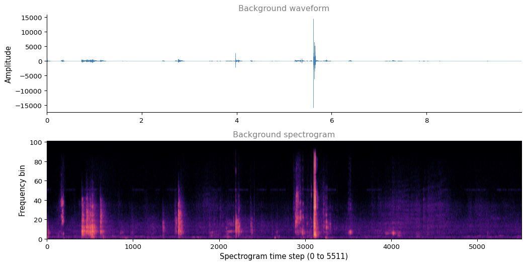
so n_freq = 101 and Tx = 5511

Those two numbers, 101 and 5,511, are what the model’s input layer expects, and they fall out of the spectrogram settings rather than being chosen directly.

One quirk is worth naming, because it affects how these plots are labeled. graph_spectrogram passes Fs=8000 while the audio is recorded at 44,100 Hz. That mismatch does more than mislabel an axis. Matplotlib’s specgram defaults to a power spectral density with scale_by_freq=True, so Fs divides the returned values as well as setting both physical axes. Dividing by 8,000 rather than by 44,100 makes the returned array larger by a factor of \(44100/8000 = 5.5125\) than the true rate would give. None of this changes the array’s shape, and the value must stay at 8,000 regardless, because the pretrained weights were fitted to spectrograms computed exactly this way. What it does mean is that the printed hertz and second axes would be wrong by a factor of about 5.5, so the plots below label the axes in frequency bins and time steps instead.

Ten seconds of background noise as a waveform and as a spectrogram. The model reads the lower panel, which is 5,511 time steps wide and 101 frequency bins tall.

Building One Training Example

To make one example, take a background clip, insert between zero and four activate clips at random positions, insert between zero and two negative clips, and record where each activate ended. Because the insertions are deliberate, the labels are known exactly, which is the whole reason for synthesizing rather than recording.

Clips must not land on top of each other, so the first thing needed is an overlap test. Two segments overlap when one starts before the other ends and ends after the other starts.

def is_overlapping(segment_time, previous_segments):
    """Does this segment collide with any already placed?"""
    start, end = segment_time
    for previous_start, previous_end in previous_segments:
        if start <= previous_end and end >= previous_start:
            return True
    return False


print("Overlap 1 =", is_overlapping((950, 1430), [(2000, 2550), (260, 949)]))
print("Overlap 2 =", is_overlapping((2305, 2950),
                                    [(824, 1532), (1900, 2305), (3424, 3656)]))

Overlap 1 = False
Overlap 2 = True

The first is False, since (950, 1430) sits in the gap between the two existing segments. The second is True, and only just, because it starts at 2305 and an existing segment ends at exactly 2305. The comparison is inclusive on both sides, so touching counts as overlapping.

Placing a clip means picking a random start that leaves room for the whole clip, retrying if it collides, and giving up after a few attempts rather than looping forever on a crowded clip.

def get_random_time_segment(segment_ms):
    """A random (start, end) in milliseconds that fits inside ten seconds."""
    start = np.random.randint(low=0, high=10000 - segment_ms)
    return (start, start + segment_ms - 1)


def insert_audio_clip(background, clip, previous_segments):
    """Overlay a clip at a free random position, or give up and return as is."""
    segment_ms = duration_ms(clip, rate)
    segment_time = get_random_time_segment(segment_ms)

    retry = 5
    while is_overlapping(segment_time, previous_segments) and retry >= 0:
        segment_time = get_random_time_segment(segment_ms)
        retry -= 1

    if not is_overlapping(segment_time, previous_segments):
        previous_segments.append(segment_time)
        return overlay(background, clip, segment_time[0], rate), segment_time
    # crowded clip, so leave the background alone and flag it with a sentinel
    return background, (10000, 10000)

Before moving on, look at what insert_audio_clip actually returns, since the autograder checked its behavior in both the ordinary and the crowded case.

np.random.seed(5)
probe_bg = apply_gain(backgrounds[0], -20)
placed, times = probe_bg, []
for clip in activates[:3]:
    placed, when = insert_audio_clip(placed, clip, times)
    print(f"  clip of {duration_ms(clip, rate):>4} ms placed at {when}, "
          f"span {when[1] - when[0] + 1} ms")

print()
print("segments recorded:", times)
print("audio length unchanged:", len(placed) == len(probe_bg))
# int16 is asymmetric, so test the two bounds separately
print("samples stay inside int16:",
      int(placed.min()) >= -32768 and int(placed.max()) <= 32767,
      f"(range {int(placed.min())} to {int(placed.max())})")

# a clip that cannot fit returns the background untouched and a sentinel
crowded = [(0, 9999)]
unchanged, sentinel = insert_audio_clip(probe_bg, activates[0], crowded)
print("when no free slot exists, the returned time is", sentinel)
print("and the background comes back untouched:",
      bool(np.array_equal(unchanged, probe_bg)))

  clip of  721 ms placed at (2915, 3635), span 721 ms
  clip of  731 ms placed at (4079, 4809), span 731 ms
  clip of 1741 ms placed at (7286, 9026), span 1741 ms

segments recorded: [(2915, 3635), (4079, 4809), (7286, 9026)]
audio length unchanged: True
samples stay inside int16: True (range -32768 to 32767)
when no free slot exists, the returned time is (10000, 10000)
and the background comes back untouched: True

The sentinel (10000, 10000) is how a failed insertion is signaled. It sits past the end of the ten second clip, so the label step it maps to falls outside \(T_y\) and insert_ones leaves the labels alone, which is exactly what should happen when nothing was inserted.

Two edge cases in is_overlapping are worth pinning down as well.

print("touching at a single point counts as overlapping:",
      is_overlapping((100, 200), [(200, 300)]))
print("new segment inside an existing one:",
      is_overlapping((150, 160), [(100, 300)]))
print("existing segment inside the new one:",
      is_overlapping((100, 300), [(150, 160)]))
print("no previous segments at all:", is_overlapping((100, 200), []))

touching at a single point counts as overlapping: True
new segment inside an existing one: True
existing segment inside the new one: True
no previous segments at all: False

Containment counts either way round, which matters because the two cases arrive by different routes. A short clip can land inside the span of a long one already placed, and a long clip can swallow a short one.

A successful insertion around an already occupied interval should change the audio, not just the bookkeeping, and it should get there by rejecting candidates that collide. Block off the first 4,400 ms so the retry loop has real work to do, and watch it run.

occupied = [(0, 4400)]

# replay the same draws the insertion will make, to see what it rejects
np.random.seed(5)
rejected, candidate, retry = [], get_random_time_segment(721), 5
while is_overlapping(candidate, occupied) and retry >= 0:
    rejected.append(candidate)
    candidate = get_random_time_segment(721)
    retry -= 1
print(f"rejected {len(rejected)} colliding candidates:", rejected)
print("accepted:", candidate)

# now the real call, from the same seed, so it follows the same path
np.random.seed(5)
before = apply_gain(backgrounds[1], -20)
after, placed_at = insert_audio_clip(before, activates[0], occupied)

print()
print("placed at:", placed_at, "which clears the occupied (0, 4400)")
print("the audio actually changed:", not np.array_equal(after, before))
print("segments now recorded:", occupied)
print("returned types:", type(after).__name__, "and", type(placed_at).__name__)

rejected 4 colliding candidates: [(2915, 3635), (2254, 2974), (4079, 4799), (3046, 3766)]
accepted: (7286, 8006)

placed at: (7286, 8006) which clears the occupied (0, 4400)
the audio actually changed: True
segments now recorded: [(0, 4400), (7286, 8006)]
returned types: ndarray and tuple

Four candidates landed inside the blocked interval and were thrown away before the fifth cleared it. The loop is more patient than that in the worst case. It draws one candidate up front, then redraws while retry counts down from 5 through 0, so it can evaluate seven positions in all. If every one of them collides the clip is simply dropped, which is where the (10000, 10000) sentinel above comes from.

Now the labels. When an activate finishes at some millisecond, the fifty output steps strictly after that moment are set to 1. Labeling only the single step where the word ends would leave one positive against 1,374 negatives, which is a hopelessly imbalanced target. Fifty steps is the hack from the lecture, widening the target without moving it.

def insert_ones(y, segment_end_ms):
    """Set the 50 output steps after `segment_end_ms` to 1."""
    _, Ty = y.shape
    segment_end_y = int(segment_end_ms * Ty / 10000.0)
    if segment_end_y < Ty:
        for i in range(segment_end_y + 1, segment_end_y + 51):
            if i < Ty:
                y[0, i] = 1
    return y


arr1 = insert_ones(np.zeros((1, Ty)), 9700)
insert_ones(arr1, 4251)          # a second word ending, so two runs of ones
print("sanity checks:", arr1[0][1333], arr1[0][634], arr1[0][635])

sanity checks: 0.0 1.0 0.0

A word that ends near the very end of the clip cannot get all fifty of its label steps, and the function truncates rather than running off the end.

for end_ms in (9700, 9990, 10000):
    labels = insert_ones(np.zeros((1, Ty)), end_ms)
    step = int(end_ms * Ty / 10000.0)
    print(f"  word ending at {end_ms:>5} ms -> output step {step:>4}, "
          f"{int(labels.sum()):>2} steps labeled 1")

  word ending at  9700 ms -> output step 1333, 41 steps labeled 1
  word ending at  9990 ms -> output step 1373,  1 steps labeled 1
  word ending at 10000 ms -> output step 1375,  0 steps labeled 1

The last row is the boundary. A word ending at exactly 10,000 ms maps to step 1,375, which is not less than \(T_y\), so no labels are set at all.

Read the earlier three checks against the rule. The word ending at 9,700 ms maps to output step 1,333, and that step itself stays 0 because the ones start after it. The word ending at 4,251 ms maps to step 584, so steps 585 through 634 are 1, which is why index 634 is 1 and index 635, the fifty-first step, is back to 0.

With those pieces, one training example is a short recipe. Lower the background so the inserted words stand out, place the clips, label after each activate, normalize the whole thing to a standard loudness, and take the spectrogram.

def create_training_example(background, activates, negatives, Ty):
    """Synthesize one ten second example and its label vector."""
    background = apply_gain(background, -20)      # lower the background volume
    y = np.zeros((1, Ty))
    previous_segments = []

    number_of_activates = np.random.randint(0, 5)
    for i in np.random.randint(len(activates), size=number_of_activates):
        background, segment_time = insert_audio_clip(
            background, activates[i], previous_segments)
        y = insert_ones(y, segment_end_ms=segment_time[1])

    number_of_negatives = np.random.randint(0, 3)
    for i in np.random.randint(len(negatives), size=number_of_negatives):
        background, _ = insert_audio_clip(
            background, negatives[i], previous_segments)

    background = match_target_amplitude(background, -20.0)
    return graph_spectrogram(background), y, background


np.random.seed(18)
x, y, audio = create_training_example(backgrounds[0], activates, negatives, Ty)
print("x shape:", x.shape, " y shape:", y.shape)
print("output steps labeled 1:", int(y.sum()), f"out of {Ty}")
print(f"labels only ever 0 or 1: {set(np.unique(y)) <= {0.0, 1.0}}")
print(f"spectrogram values all positive: {bool(x.min() > 0)}, "
      f"min {x.min():.3g}")
print(f"spectrogram Frobenius norm: {np.linalg.norm(x):,.2f}")
print("returned types:", type(x).__name__, "and", type(y).__name__)
print(f"that is {100 * y.mean():.1f}% positive, so the target is still "
      f"imbalanced even after widening")

x shape: (101, 5511)  y shape: (1, 1375)
output steps labeled 1: 100 out of 1375
labels only ever 0 or 1: True
spectrogram values all positive: True, min 9.18e-14
spectrogram Frobenius norm: 38,078,999.36
returned types: ndarray and ndarray
that is 7.3% positive, so the target is still imbalanced even after widening

The notebook records a norm of 39,745,552.52 for its own example. This page gets a different figure, and the reason is not a bug. A genuinely different example is being synthesized, because the clips load in sorted rather than filesystem order and the seeded draws therefore select different recordings. Flooring is not the cause. audioop already floored, so the quantization here restores the original behavior rather than departing from it, and switching it to rounding moves the norm by only a few hundred out of a difference of about 1.67 million.

What the stripped check was really protecting still holds. The labels take only the values 0 and 1, and the spectrogram is positive throughout, with a measured minimum of about \(9 \times 10^{-14}\). Note that positivity is a measurement on this example rather than a guarantee, since a power spectral density is non-negative and could in principle contain an exact zero.

Plot the example against its labels. The steps of y that are 1 should sit just after each inserted activate burst. The inserted negative words also show as speech in the spectrogram and deliberately get no pulse.

Listen to what was just built. The activate clips should be audible over the background, and each one is what produces a pulse in the label below.

display(play(audio, rate, 'synthesized_example.wav'))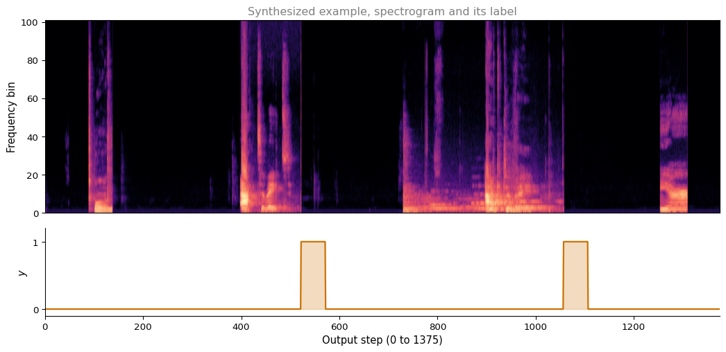

One synthesized training example. The upper panel is the spectrogram the model reads, and the lower panel is the label it must produce, which rises to 1 for fifty steps immediately after each inserted activate.

Model

The network is a 1D convolution followed by two GRU layers and a time-distributed dense output.

The convolution does two jobs. It extracts local features from the spectrogram, and its stride of 4 is what turns 5,511 input steps into 1,375 output steps, which is where \(T_y\) actually comes from. The GRUs then carry context along the sequence, and the final dense layer, applied at every step, emits one probability per output position.

import keras
from keras.layers import (Activation, BatchNormalization, Conv1D, Dense,
                          Dropout, GRU, Input, TimeDistributed)
from keras.models import Model

keras.utils.set_random_seed(1)


def modelf(input_shape):
    """The trigger word model. One Conv1D, two GRUs, a dense output per step."""
    X_input = Input(shape=input_shape)

    X = Conv1D(196, kernel_size=15, strides=4)(X_input)
    X = BatchNormalization()(X)
    X = Activation('relu')(X)
    X = Dropout(0.8)(X)

    X = GRU(units=128, return_sequences=True)(X)
    X = Dropout(0.8)(X)
    X = BatchNormalization()(X)

    X = GRU(units=128, return_sequences=True)(X)
    X = Dropout(0.8)(X)
    X = BatchNormalization()(X)
    X = Dropout(0.8)(X)

    X = TimeDistributed(Dense(1, activation="sigmoid"))(X)
    return Model(inputs=X_input, outputs=X)


model = modelf(input_shape=(Tx, n_freq))

The autograder compared this against a stored summary. Here is what it was checking, printed out, first the shapes and then the layer configuration it also asserted.

print("total parameters:", f"{model.count_params():,}")
print("input shape: ", model.input.shape)
print("output shape:", model.output.shape)
print()
print("every layer in build order:")
for layer in model.layers:
    print(f"  {type(layer).__name__:20} {str(tuple(layer.output.shape)):22}"
          f"{layer.count_params():>8,} params")

total parameters: 523,329
input shape:  (None, 5511, 101)
output shape: (None, 1375, 1)

every layer in build order:
  InputLayer           (None, 5511, 101)            0 params
  Conv1D               (None, 1375, 196)      297,136 params
  BatchNormalization   (None, 1375, 196)          784 params
  Activation           (None, 1375, 196)            0 params
  Dropout              (None, 1375, 196)            0 params
  GRU                  (None, 1375, 128)      125,184 params
  Dropout              (None, 1375, 128)            0 params
  BatchNormalization   (None, 1375, 128)          512 params
  GRU                  (None, 1375, 128)       99,072 params
  Dropout              (None, 1375, 128)            0 params
  BatchNormalization   (None, 1375, 128)          512 params
  Dropout              (None, 1375, 128)            0 params
  TimeDistributed      (None, 1375, 1)            129 params

conv = model.layers[1]
gru1, gru2 = model.layers[5], model.layers[8]
dropouts = [l for l in model.layers if type(l).__name__ == 'Dropout']
head = model.layers[-1].layer          # the Dense inside TimeDistributed

print("Conv1D: kernel_size", conv.kernel_size[0], " strides", conv.strides[0],
      " padding", repr(conv.padding), " activation",
      conv.activation.__name__)
print("kernel initializer:", type(conv.kernel_initializer).__name__)
print("GRU return_sequences:", gru1.return_sequences, gru2.return_sequences)
print("Dropout rates:", [l.rate for l in dropouts])
print("output Dense activation:", head.activation.__name__)

Conv1D: kernel_size 15  strides 4  padding 'valid'  activation linear
kernel initializer: GlorotUniform
GRU return_sequences: True True
Dropout rates: [0.8, 0.8, 0.8, 0.8]
output Dense activation: sigmoid

Three of those are defaults worth noticing rather than skimming. The padding is valid, so the convolution shortens the sequence rather than preserving its length, which is exactly how 5,511 becomes 1,375. The convolution’s own activation is linear, because the ReLU is applied as a separate layer after the batch normalization rather than inside the convolution. And the kernel initializer is Glorot uniform, which is Keras’s default rather than a choice this model makes.

Two things in that table matter. The Conv1D collapses the time axis from 5,511 to 1,375 in one step, and it holds 297,136 of the 523,329 parameters, more than half the model. Everything after it works at the output resolution.

WarningDropout of 0.8 is unusually aggressive

Four dropout layers at rate 0.8 means each drops 80 percent of its units during training, far heavier than the 0.2 to 0.5 typical elsewhere. The notebook does not explain the choice, so treat what follows as a plausible reading rather than something the source states. Every example is synthesized from ten activate recordings, ten negatives and two backgrounds, which is very little genuine variety, and a model with 523,329 parameters could fit those particular voices and that particular noise closely. Heavy dropout is the usual response to exactly that risk.

The notebook fine-tunes this model for one epoch on 32 synthesized examples at a learning rate of \(10^{-6}\), then evaluates on a 25-example development set. Neither is rerun here, the first because synthesizing 32 examples at render time is expensive for what one epoch at that learning rate buys, and the second because its arrays are not hosted. For the record, the notebook reports a training accuracy of 0.9467 after that epoch and a development set accuracy of 0.9240.

Since the fine-tuning is skipped, load the trained weights directly.

model.load_weights(WEIGHTS_FILE)
print("loaded pretrained weights into the rebuilt architecture")

loaded pretrained weights into the rebuilt architecture

NoteWhat the training step would have looked like

Left here for reference. Note learning_rate rather than the original lr, and that X and Y would be the 32 synthesized examples stacked, not a loaded array.

from keras.optimizers import Adam

# freeze the batch norm layers before fine tuning a pretrained model
model.layers[2].trainable = False
model.layers[7].trainable = False
model.layers[10].trainable = False

opt = Adam(learning_rate=1e-6, beta_1=0.9, beta_2=0.999)
model.compile(loss='binary_crossentropy', optimizer=opt, metrics=["accuracy"])
model.fit(X, Y, batch_size=16, epochs=1)

Detecting the Trigger Word

Detection normalizes the clip toward a standard loudness, takes its spectrogram, transposes it so time runs along the first axis, and predicts. The normalization is not optional. Every training example was normalized toward \(-20\) dBFS, so a much quieter recording lands outside the range of input scales the model ever saw, and its peak probability falls far enough that it fires on nothing.

Note that \(-20\) dBFS is a target rather than a guarantee. Raising a clip’s level can push samples past the 16-bit range, and the saturation that follows costs some of the gain, so the achieved loudness lands near the target rather than on it. The diagnostic below shows a request for \(-20.0\) arriving at \(-20.62\).

def detect_triggerword(path):
    """Return the model's per-step probability curve for one audio file."""
    rate_in, samples = load_wav(path)
    samples = match_target_amplitude(samples, -20.0)     # required, not cosmetic
    x = graph_spectrogram(samples).swapaxes(0, 1)        # (Tx, n_freq)
    return model.predict(np.expand_dims(x, axis=0), verbose=0)[0, :, 0], samples


for name in DEV_FILES:
    probs, _ = detect_triggerword(name)
    crossings = int(np.sum((probs[1:] > 0.5) & (probs[:-1] <= 0.5)))
    print(f"  {name.split('/')[-1]}: peak probability {probs.max():.3f}, "
          f"crosses 0.5 {crossings} time(s)")

  1.wav: peak probability 0.701, crosses 0.5 1 time(s)
  2.wav: peak probability 0.688, crosses 0.5 3 time(s)

Here is the first development clip as recorded, before any of that.

display(Audio(filename=DEV_FILES[0]))

That claim about normalization is easy to test rather than assert. Run the same clip both ways.

_, raw = load_wav(DEV_FILES[0])
raw_spec = graph_spectrogram(raw).swapaxes(0, 1)
raw_probs = model.predict(np.expand_dims(raw_spec, axis=0), verbose=0)[0, :, 0]
norm_probs, _ = detect_triggerword(DEV_FILES[0])

# report the loudness actually achieved, since clipping pulls it off target
normalized = match_target_amplitude(raw, -20.0)
raw_hits = int(np.sum((raw_probs[1:] > 0.5) & (raw_probs[:-1] <= 0.5)))
norm_hits = int(np.sum((norm_probs[1:] > 0.5) & (norm_probs[:-1] <= 0.5)))

print(f"  as recorded, {dbfs(raw):>7.2f} dBFS: peak probability "
      f"{raw_probs.max():.3f}, crossings {raw_hits}")
print(f"  after asking for -20.0, {dbfs(normalized):>7.2f} dBFS: peak "
      f"probability {norm_probs.max():.3f}, crossings {norm_hits}")

  as recorded,  -35.76 dBFS: peak probability 0.286, crossings 0
  after asking for -20.0,  -20.62 dBFS: peak probability 0.701, crossings 1

Each upward crossing of the threshold is a candidate rather than a finished detection, and turning candidates into chimes is the last section’s job. Plot the curve against the spectrogram to see where the candidates land.

Detection on a held-out development clip. The probability curve stays near zero through the background and the negative words, and spikes only where the trigger word finishes.

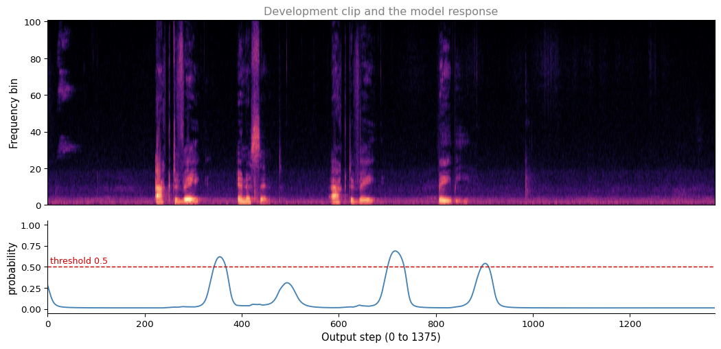
The last step is to act on a detection. A single upward crossing is too twitchy, since the probability wobbles across the threshold as it rises, so a crossing is treated as a candidate rather than a detection. The scan counts consecutive steps above the threshold, fires once that count passes 20, and then jumps forward to the next multiple of 75 to avoid firing repeatedly inside one long run.

Two details of the notebook’s implementation are worth reading carefully, since they are kept here for fidelity and neither behaves quite as the description suggests. The counter is incremented and tested before the current step’s probability is examined, so 20 high steps followed by one low step still fire. And the jump goes to the next global multiple of 75 rather than 75 steps forward, so a run that begins just before a boundary can still produce two chimes. On the development clip below, three threshold crossings produce two chimes.

def chime_on_activate(path, probs, threshold=0.5):
    """Chime once the probability has held above the threshold for 20 steps."""
    rate_in, samples = load_wav(path)
    _, chime = load_wav(CHIME_FILE)
    duration_s = len(samples) / rate_in

    consecutive, fired, i = 0, 0, 0
    while i < Ty:
        consecutive += 1
        if consecutive > 20:
            samples = overlay(samples, chime,
                              (i / Ty) * duration_s * 1000, rate_in)
            fired += 1
            consecutive = 0
            i = 75 * (i // 75 + 1)      # skip to the next 75-step block
            continue
        if probs[i] < threshold:
            consecutive = 0
        i += 1
    return samples, fired


output, fired = chime_on_activate(DEV_FILES[1], probs)

# write somewhere temporary, since rendering runs in the page's own directory
out_path = os.path.join(tempfile.gettempdir(), 'chime_output.wav')
write_wav(out_path, output, rate)
print(f"inserted {fired} chime(s) into a "
      f"{duration_ms(output, rate) / 1000:.0f} second clip")
print("wrote", out_path, f"({os.path.getsize(out_path) / 1e6:.1f} MB)")

display(Audio(filename=out_path))

inserted 2 chime(s) into a 10 second clip
wrote /var/folders/16/sty8fwps4996_1wfn71yphsh0000gp/T/chime_output.wav (1.8 MB)

The chimes land where the probability curve crossed and held. That completes the course’s pipeline. Synthesize labeled data, train on it, then act on the output. This page executes the first and third of those and loads the course’s weights in place of the second.

NoteWhat You Should Remember

• Synthesizing a dataset gives you exact labels for free, which is the whole reason this task is tractable without hand-labeled speech.
• Four time units coexist here, 441,000 samples, 10,000 milliseconds, 5,511 spectrogram steps and 1,375 output steps, and most of the code is conversion between them.
• The convolution’s stride is what maps \(T_x\) to \(T_y\), so the output resolution is a consequence of the architecture rather than a free choice.
• Labeling fifty steps after each trigger word instead of one is a deliberate hack against class imbalance, and even after it the target is still mostly zeros.
• Input normalization is part of the model. A clip at the wrong loudness silently produces no detections rather than an error.
• pydub is not needed for any of this. Loading, gain, overlay and export are a few lines of NumPy over the standard library wave module.

Review Questions

1. Where does \(T_y = 1375\) come from? It is not chosen directly anywhere in the code.

Answer

From the convolution. The input has \(T_x = 5511\) steps, and Conv1D(196, kernel_size=15, strides=4) slides a width-15 window with a stride of 4, giving \(\lfloor (5511 - 15)/4 \rfloor + 1 = 1375\) output positions. Every layer after the convolution works at that resolution, so the shape of the label vector is fixed by the architecture. Changing the stride or the kernel size would change how many predictions the model makes per clip.

---

1. Why label fifty output steps after each activate rather than the single step where it ends?

Answer

Class imbalance. A clip has 1,375 output steps and at most four trigger words, so labeling one step each would give at most four positives against at least 1,371 negatives. A model that predicted 0 everywhere would already score above 99.7 percent accuracy, and there would be almost no gradient pushing it to do anything else. Widening each positive to fifty steps raises the share of ones enough for the model to learn something, without moving where the ones sit.

It is worth naming this as the hack it is. Nothing about the task says the trigger word lasts fifty output steps. The number is a training convenience.

---

1. detect_triggerword normalizes the clip to \(-20\) dBFS before taking the spectrogram. What happens if you skip that?

Answer

The probabilities collapse and the model detects nothing, while raising no error at all. Every training example was normalized toward \(-20\) dBFS by create_training_example, so the model only ever saw spectrograms at roughly that loudness. A quieter clip shifts the spectrogram scale downward, which is an input distribution the model was never trained on, and its peak output stays below the threshold. The shift is not uniform, since clipping and quantization mean a minority of bins and steps move the other way, but the overall scale and the peak both drop. The page measures this rather than asserting it, finding a peak of 0.286 and no threshold crossings at \(-35.76\) dBFS against 0.701 and one crossing after normalizing.

Note the word roughly. Clipping means the normalization lands near \(-20\) dBFS rather than exactly on it, so the training distribution is a narrow band of loudness rather than a single value.

This is the failure mode worth internalizing, because it looks like a model problem and is actually a preprocessing problem. The normalization is as much a part of the model as any layer.

---

1. chime_on_activate fires once its consecutive-step counter passes 20, then jumps to the next multiple of 75. What does each mechanism buy, and what exactly does the counter count?

Answer

They guard against two different failures. The counter guards against noise, demanding sustained evidence rather than one lucky sample. Be precise about what it counts, though. The loop increments and tests it before checking the current step’s probability, and a sub-threshold value only resets it afterwards. So it is not strictly a count of steps above the threshold. Twenty high steps followed by one low step still fire, on the low step itself, because the counter reaches 21 before that low value gets its chance to reset it. The practical effect is a firing rule of roughly 20 steps of sustained evidence, with an off-by-one at the boundary that the notebook’s code has and this page keeps for fidelity.

The block jump reduces double counting. A single spoken activate produces a run of high probability roughly fifty steps wide, and after firing partway through that run the counter would otherwise refill and fire again on the same word. Jumping forward skips most of the remaining run. It does not eliminate the problem, because the jump lands on the next global multiple of 75 rather than 75 steps ahead, so a run starting just before a boundary can be cut short enough to fire twice.

---

1. The model uses dropout at rate 0.8 in four places. Why so aggressive, and what might that tell you about the dataset?

Answer

The notebook does not say, so what follows is a reading rather than a quotation. The dataset has very little genuine variety. Every example is built from the same ten activate recordings, the same ten negatives and two background clips, so a model with 523,329 parameters could fit those specific voices and that specific noise closely while generalizing poorly to a new speaker.

Dropping 80 percent of units is the standard response to that risk, since it stops the network leaning on a few units that have latched onto one speaker. Read the rate as a signal about the data rather than about the architecture. More real recordings would be the better fix, and heavy dropout is what you reach for when you cannot get them.