Train an LSTM on a jazz corpus using the Keras functional API with shared layers, then feed its own predictions back to generate and play a new solo.
Published
Aug 25, 2026
This is the last assignment of the week, and the one where the model produces something you can listen to. The task is to generate a jazz solo. A corpus of performed jazz is chopped into short sequences of musical values, an LSTM learns to predict the next value from the ones before it, and a second model built from the same trained weights runs that prediction forward on its own output until it has written a solo.
By the end of this lab you will be able to
apply an LSTM to a music generation task,
build a model with shared layers using the Keras functional API,
write a time-step loop by hand when Keras cannot supply the inputs in advance,
generate a sequence by feeding a model its own predictions.
Two things separate this from the character-level model built on the previous page. That one was NumPy from end to end, and this one is Keras. That one predicted a character at every time step from a sequence handed to it in full, and this one has to generate values it has not seen yet, which means the input at step \(t\) is the output from step \(t-1\) and Keras cannot vectorize the loop for you.
ImportantUpdated From the Original Assignment
The original assignment was written against TensorFlow 2.3, Keras 2, NumPy 1.x, and music21 5. None of that code runs on the current stack, so this page is ported to TensorFlow 2.21, Keras 3.15, NumPy 2.4, and music21 10.5, updated on 2026-08-25. Seven changes were needed.
Keras 3 renamed the recurrent layer call argument from inputs to sequences. The lab’s LSTM_cell(inputs=x, initial_state=[a, c]) raises TypeError: missing a required argument: 'sequences'. The cell is called positionally here instead.
Raw TensorFlow ops cannot be applied to a symbolic tensor in Keras 3. The original called tf.math.argmax and tf.one_hot directly on a layer output while building the graph. They are wrapped in a Lambda layer here, using keras.ops so the layer stays backend-agnostic.
Keras 3 requires one metric per output. The model has 30 outputs, so metrics=['accuracy'] is rejected and becomes metrics=['accuracy'] * Tx.
Adam(lr=0.01, decay=0.01) is rejected by Keras 3. The argument is learning_rate, and decay was removed in favor of learning rate schedules.
np.bool was removed in NumPy 1.24. The one-hot arrays use the builtin bool.
music21 10 parses MIDI differently.Metadata now occupies index 0 of the parsed score, which shifts every part index by one, MIDI import no longer groups notes into Voice objects, getElementsByClass returns a StreamIterator that cannot be appended to a stream, and .flat became .flatten(). The parsing step is reproduced inline in modernized form rather than imported.
pydub is unmaintained and does not run on Python 3.13, because audioop was removed from the standard library in PEP 594. The lab used it only to turn the generated MIDI into audible sine tones, which is about twenty lines of NumPy, written out below.
One result changed as a consequence. The 2019 parse produced 90 distinct musical values and this one produces 87, because the old two-Voice merge picked up a handful of simultaneous notes that the current importer represents differently. The network is sized from the data rather than from a hardcoded 90, so everything downstream is unaffected. The corpus, the architecture, the hyperparameters, and the generation procedure are otherwise unchanged.
Packages
Alongside the usual imports, this lab needs music21 for reading and writing MIDI and mido for turning the result into audio.
Two of the assignment’s helper modules are imported unchanged, because they are pure music theory and needed no migration. grammar.py converts between a stream of notes and the text grammar the model learns, and qa.py holds the post-processing that cleans up a generated line.
grammar.py (15 KB) and qa.py (3 KB), the two helper modules this page imports unchanged.
30s_seq.mp3 (460 KB), thirty seconds of the training corpus.
30s_trained_model.mp3 (470 KB), thirty seconds generated by a fully trained reference model.
preprocess.py, music_utils.py and data_utils.py, the original versions of the modules this page replaces. They are here for comparison and do not run on the current stack.
Problem Statement
The training data is a recording of a jazz performance. Here are thirty seconds of it.
The model never sees audio. It sees musical values, which is the representation the assignment’s preprocessing produces from the MIDI file. A value is informally a note, meaning a pitch and a duration, but it records both of those relative to their surroundings rather than absolutely. A real value from this corpus is A,0.250,<m2,P-4>, and it has three fields.
A is the tone type, which says how the note sits against the chord playing underneath it. __is_approach_tone in grammar.py marks a note as an approach tone when its pitch class sits exactly one semitone above or below one of the chord pitches. It does not look at what comes next, so nothing in this implementation requires the note to actually resolve. The other types are C for a chord tone, S for a scale tone, X for an arbitrary tone, and R for a rest. The 87 distinct values in this corpus break down as 40 chord tones, 21 scale tones, 15 rests, 10 approach tones and 1 arbitrary tone.
0.250 is the duration in quarter notes, so a quarter of a beat.
<m2,P-4> is a pair of intervals measured from the previous note, a minor second up and a perfect fourth down. It bounds a window the pitch may fall in rather than fixing one pitch, which grammar.py produces by taking the actual interval and widening it by a minor third in each direction.
Nothing in that value names a pitch. The solo is stored as a sequence of moves, relative to the harmony for its type and to the previous note for its size, so the same learned pattern replayed over a different chord lands on different notes and still belongs to the harmony. That property is what makes the generation step later in this lab work at all.
Reading the Corpus
The corpus is parsed in four steps. The MIDI file is read into parts, the solo section is cut out of the melody part and the chord part, both are grouped into measures, and each measure of melody is converted to grammar text against the chords underneath it.
The parsing below is the modernized replacement for the assignment’s __parse_midi. The two constants are the offsets of the accompanied solo inside the recording, which the original lab identified by hand.
from collections import OrderedDictfrom itertools import groupbySOLO_START, SOLO_END =476, 548# offsets of the accompanied solo, in quarter notesMELODY_PART, CHORD_PART =6, 1# part indices, shifted by one under music21 10def extract_solo(part):"""Cut the solo window out of a part, keeping every element at its real offset.""" out = stream.Part()for element in part.flatten().getElementsByOffset(SOLO_START, SOLO_END, includeEndBoundary=True): out.insert(element.offset - SOLO_START, element)return outdef group_by_measure(elements):"""Group elements into bars of four quarter notes, keyed by bar number.""" grouped = OrderedDict()for bar, items in groupby([(int(e.offset /4), e) for e in elements], lambda pair: pair[0]): grouped[bar] = [item[1] for item in items]return grouped
extract_solo uses insert rather than append, which is the detail that makes the whole thing work. Appending to a music21 stream places each element after the previous one and renumbers its offset, which would destroy the timing and let two notes that are played together become two notes played in sequence. insert puts each element at an offset you choose, so subtracting SOLO_START shifts the solo to begin at zero while every note keeps its position relative to the others.
score = converter.parse(DATA +"original_metheny.mid")melody = extract_solo(score[MELODY_PART])for element in melody:if element.quarterLength ==0.0: element.quarterLength =0.25# give zero-length notes a real durationchord_stream = extract_solo(score[CHORD_PART])chord_stream.removeByClass(note.Rest) # keep only the chords, drop single notes and restschord_stream.removeByClass(note.Note)measures = group_by_measure(melody.notesAndRests)chords = group_by_measure(chord_stream)print("parts in the score:", len(score))print("melody part:", score[MELODY_PART].partName, "| chord part:", score[CHORD_PART].partName)print("melody groups:", len(measures), "| chord groups:", len(chords))
parts in the score: 20
melody part: Guitar | chord part: Piano
melody groups: 19 | chord groups: 19
Nineteen groups on each side. Eighteen of them are real bars of the accompanied solo, and the nineteenth is a boundary artifact, as the next step explains.
Each bar of melody is now converted into grammar text. parse_melody is the unchanged helper, and it needs the melody and the chords of the same bar wrapped in streams.
def measure_to_stream(elements):"""Wrap a list of elements back into a Voice at their own offsets.""" voice = stream.Voice()for element in elements: voice.insert(element.offset, element)return voicebars =sorted(set(measures) &set(chords))abstract_grammars = [ parse_melody(measure_to_stream(measures[bar]), measure_to_stream(chords[bar]))for bar in bars[:-1] # drop the trailing boundary group]corpus = [value for grammar in abstract_grammars for value in grammar.split(' ')]values =sorted(set(corpus))n_values =len(values)value_to_index = {value: index for index, value inenumerate(values)}index_to_value = {index: value for index, value inenumerate(values)}print("corpus length:", len(corpus))print("number of distinct values:", n_values)print("first grammar:", abstract_grammars[0][:70], "...")
corpus length: 211
number of distinct values: 87
first grammar: C,0.667 C,0.333,<P1,d-5> R,0.333 C,0.750,<P4,m-2> C,0.333,<d1,P-5> R,0 ...
One of the nineteen groups is discarded, and which one matters. The solo window spans offsets 476 to 548, which is 72 quarter notes, or exactly 18 bars of four. Grouping with includeEndBoundary=True produces a nineteenth group holding whatever sits precisely on the closing offset, which here is a single element against the ten to eighteen in every real bar. That trailing group is the artifact, so it is the one dropped, leaving the 18 bars the assignment also ends up with.
The original code reaches the same 18 from the other end. It removed the trailing group with del chords[len(chords) - 1], and then skipped index 0 with range(1, len(measures)), because it grouped the whole stream including the instrument, key signature, time signature and metronome mark it had inserted, which collected into a metadata bucket at offset zero. This parse groups melody.notesAndRests only and never builds that bucket, so skipping index 0 here would throw away a real bar of music.
The corpus is 211 values long and uses 87 distinct ones. n_values is read from the data here rather than hardcoded, which is the change that lets this page keep working after the music21 upgrade moved the count off the 90 the original assignment printed.
Building the Training Set
The corpus is one long sequence, so training examples are cut from it at random. Sixty snippets of thirty consecutive values each become \(X\), and \(Y\) is the same thing shifted one step earlier, so that predicting \(Y\) at step \(t\) means predicting the value that follows \(X\) at step \(t\).
m =60# number of training examplesTx =30# time steps per examplen_a =64# dimension of the LSTM hidden statenp.random.seed(0)X = np.zeros((m, Tx, n_values), dtype=bool)Y = np.zeros((m, Tx, n_values), dtype=bool)for i inrange(m): start = np.random.choice(len(corpus) - Tx) snippet = corpus[start:start + Tx]for j inrange(Tx): index = value_to_index[snippet[j]]if j !=0: X[i, j, index] =1# the value at step j is an input Y[i, j -1, index] =1# and the label of the step before itY = np.swapaxes(Y, 0, 1) # (m, Tx, n_values) becomes (Tx, m, n_values)print("shape of X:", X.shape)print("shape of Y:", Y.shape)
shape of X: (60, 30, 87)
shape of Y: (30, 60, 87)
Two details in that loop are worth slowing down for.
The guard if j != 0 leaves the first time step of every example as an all-zero vector. Unlike the dinosaur names, these snippets start in the middle of a performance, so there is no meaningful first value to condition on and the model is simply given nothing at step 0.
The swap at the end turns \(Y\) from \((m, T_x, n_{\text{values}})\) into \((T_x, m, n_{\text{values}})\). That looks gratuitous until you see how the model is trained. The model has one output per time step, so Keras wants the labels as a list of \(T_x\) arrays, each holding the labels for all \(m\) examples at that step. Putting time first makes list(Y) exactly that.
Model Overview
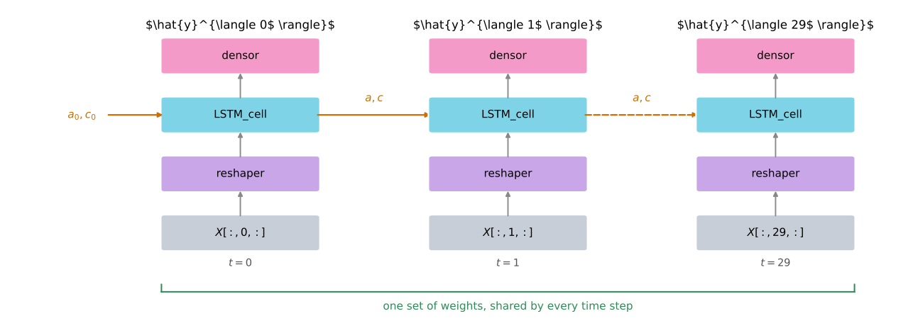
The training model unrolls an LSTM over \(T_x\) steps by hand, and every step reuses the same three layer objects.
On a small screen, scroll horizontally to inspect the complete diagram.
The training model. One slice of X enters at each step, and the same reshaper, LSTM cell and dense layer are reused across all thirty steps.
Three layer objects are created once, outside the model function, and referenced inside the loop. Referring to the same object at every step is what makes the weights shared. Creating an LSTM inside the loop would build thirty separate cells with thirty separate sets of weights, which is not a recurrent network at all.
reshaper = Reshape((1, n_values)) # (n_values,) becomes (1, n_values)LSTM_cell = LSTM(n_a, return_state=True) # returns output, hidden state, cell statedensor = Dense(n_values, activation='softmax') # one score per possible value
return_state=True is what makes the cell usable one step at a time. Without it the layer returns only its output, and the hidden and cell states needed to continue the sequence would be thrown away.
Building the Model
djmodel walks the time steps and wires the layers together. At each step it takes the slice of X for that step, reshapes it so the LSTM sees a sequence of length one, runs the cell forward carrying a and c from the previous step, and applies the dense layer to produce a prediction.
def djmodel(Tx, LSTM_cell, densor, reshaper):""" Build the training model, Tx LSTM steps sharing one set of weights. Arguments: Tx -- length of the sequences in the corpus LSTM_cell -- LSTM layer instance, shared across time steps densor -- Dense layer instance, shared across time steps reshaper -- Reshape layer instance, shared across time steps Returns: model -- a Keras model with inputs [X, a0, c0] and Tx outputs """ n_values = densor.units n_a = LSTM_cell.units# The sequence, plus the initial hidden and cell states. X = Input(shape=(Tx, n_values)) a0 = Input(shape=(n_a,), name='a0') c0 = Input(shape=(n_a,), name='c0') a = a0 c = c0# Step 1: somewhere to collect one prediction per time step. outputs = []# Step 2: walk the time steps.for t inrange(Tx):# 2.A: the values at time step t, shape (m, n_values). x = X[:, t, :]# 2.B: give it a time axis of length one, shape (m, 1, n_values). x = reshaper(x)# 2.C: one step of the LSTM, carrying the state forward. _, a, c = LSTM_cell(x, initial_state=[a, c])# 2.D: turn the hidden state into a distribution over values. out = densor(a)# 2.E: keep it. outputs.append(out)# Step 3: assemble the model. model = Model(inputs=[X, a0, c0], outputs=outputs)return modelmodel = djmodel(Tx=Tx, LSTM_cell=LSTM_cell, densor=densor, reshaper=reshaper)print("total parameters:", model.count_params())print("number of outputs:", len(model.outputs))print("shape of one output:", model.outputs[0].shape)
total parameters: 44567
number of outputs: 30
shape of one output: (None, 87)
The cell is called as LSTM_cell(x, initial_state=[a, c]), positionally. The original assignment wrote LSTM_cell(inputs=x, ...), which was correct against Keras 2 but fails on Keras 3, where the first parameter of a recurrent layer is named sequences.
Count the parameters against the architecture. The LSTM holds four gates, each with a weight matrix on the input, a weight matrix on the hidden state, and a bias, giving \(4 \times (n_{\text{values}} \times n_a + n_a \times n_a + n_a)\). The dense layer adds \(n_a \times n_{\text{values}} + n_{\text{values}}\). Nothing in that total depends on \(T_x\), because the thirty steps are the same layers used thirty times.
The model is compiled with Adam and categorical cross-entropy, and all three arguments differ from the original assignment. learning_rate replaces the Keras 2 spelling lr. metrics has to name one metric per output, because Keras 3 refuses a single metric for a thirty-output model. And decay=0.01, which Keras 3 removed outright, comes back as the learning rate schedule that argument used to be shorthand for.
# Keras 2's `decay=0.01` meant lr_t = lr_0 / (1 + 0.01 * iterations). That argument# is gone in Keras 3, and InverseTimeDecay with decay_steps=1 is the same formula.schedule = keras.optimizers.schedules.InverseTimeDecay( initial_learning_rate=0.01, decay_steps=1, decay_rate=0.01)opt = Adam(learning_rate=schedule, beta_1=0.9, beta_2=0.999)model.compile(optimizer=opt, loss='categorical_crossentropy', metrics=['accuracy'] * Tx)a0 = np.zeros((m, n_a))c0 = np.zeros((m, n_a))history = model.fit([X, a0, c0], list(Y), epochs=100, verbose=0)print(f"loss at epoch 1: {history.history['loss'][0]:.4f}")print(f"loss at epoch 100: {history.history['loss'][99]:.4f}")
loss at epoch 1:   128.2841
loss at epoch 100: 8.6887
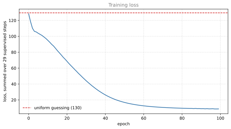
The loss reported here is a sum across outputs rather than an average, which is why it starts near 130 rather than near 4.
Count the outputs that actually contribute. The label loop writes Y[i, j - 1] for j from 1 to 29, so it fills time indices 0 through 28 and leaves index 29 all zero. Categorical cross-entropy against an all-zero target is zero, so the thirtieth output is unsupervised and contributes nothing. The baseline to compare against is therefore 29 steps, not 30. A model guessing uniformly among 87 values scores \(\ln 87 \approx 4.47\) per step, so uniform guessing over 29 supervised steps costs about 129.5, which is almost exactly where the first epoch lands.
Training loss over 100 epochs, summed across the 29 supervised time steps.
The curve drops fast and then flattens. With sixty examples drawn from a 211-value corpus, the model is partly memorizing, which is expected and is fine for this task. The goal is a model that has absorbed the style well enough to continue it, not one that generalizes to unseen jazz.
NoteWhat You Should Remember
Sequence generation needs a hand-written time-step loop, because the input at step \(t\) is not known until step \(t-1\) has produced it.
Shared weights come from referring to the same layer object inside the loop, not from any special Keras setting.
return_state=True is what lets a recurrent layer be driven one step at a time.
The parameter count of a recurrent model does not depend on the number of time steps.
Review Questions
1. Why are reshaper, LSTM_cell and densor created outside djmodel rather than inside the loop?
Answer
Because a Keras layer object owns its weights. Calling the same object thirty times reuses one weight matrix at every step, which is what makes the network recurrent and what lets it apply the patterns it learned at one position to any other. Constructing an LSTM inside the loop would create thirty independent cells with thirty independent weight sets, multiplying the parameter count by thirty and destroying the sharing that the whole architecture depends on.
1. Y is transposed to put time first, then passed as list(Y). What would happen without the swap?
Answer
The model has thirty separate outputs, so Keras expects thirty separate label arrays, one per output, each covering all sixty examples. After the swap Y has shape \((30, 60, 87)\), so list(Y) is thirty arrays of shape \((60, 87)\), which matches. Without the swap Y has shape \((60, 30, 87)\) and list(Y) would be sixty arrays of shape \((30, 87)\), so Keras would be handed sixty label sets for a model with thirty outputs and would reject the call.
1. Why does the first time step of every training example hold an all-zero vector?
Answer
Because the snippets are cut from random positions in the middle of a performance, so there is no value that reliably precedes them. The if j != 0 guard leaves step 0 empty and starts the real inputs at step 1. This differs from the dinosaur names lab only in motivation. There the zero input marked the start of a name, and here it marks that the model is being dropped into the middle of a piece with no context.
Generating Music
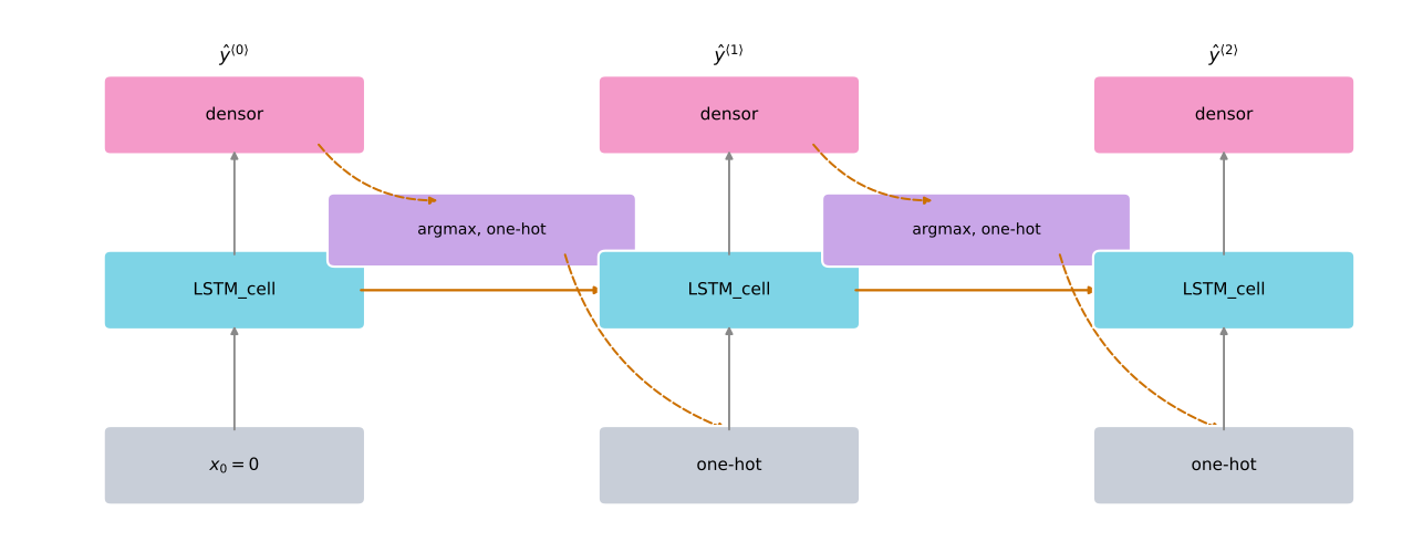
The trained weights now live inside LSTM_cell and densor. A second model is built from those same two objects, wired differently. Instead of reading a slice of a given sequence at each step, it takes its own previous prediction as the next input.
On a small screen, scroll horizontally to inspect the complete diagram.
The inference model. The prediction at one step is turned back into a one-hot input for the next, so the model writes its own continuation.
Turning a prediction back into an input takes two operations. argmax picks the index of the highest-scoring value, and one_hot turns that index back into a vector the LSTM can read. Both have to happen inside the graph, on a symbolic tensor.
This is the second place Keras 3 breaks the original code. The assignment applied tf.math.argmax and tf.one_hot directly to a layer output while building the model, which Keras 2 tolerated and Keras 3 does not. The operations go inside a Lambda layer here, written with keras.ops rather than tf so the arithmetic dispatches to whichever backend Keras is running on instead of hard-wiring TensorFlow, and with an explicit output_shape so Keras knows the shape without tracing the function. A Lambda wrapping an anonymous function is still awkward to save and reload, and a named Layer subclass would be the durable choice. Lambda is used here because it is the smallest change to the assignment’s code.
def one_hot_argmax_layer(n_values):"""A layer that turns a distribution over values into a one-hot of the argmax."""return Lambda(lambda scores: keras.ops.one_hot(keras.ops.argmax(scores, axis=-1), n_values), output_shape=(n_values,), )def music_inference_model(LSTM_cell, densor, Ty=100):""" Build the generation model from the trained LSTM_cell and densor. Arguments: LSTM_cell -- the trained LSTM layer instance densor -- the trained Dense layer instance Ty -- number of time steps to generate Returns: inference_model -- a Keras model with inputs [x0, a0, c0] and Ty outputs """ n_values = densor.units n_a = LSTM_cell.units x0 = Input(shape=(1, n_values)) a0 = Input(shape=(n_a,), name='a0') c0 = Input(shape=(n_a,), name='c0') a = a0 c = c0 x = x0# Step 1: somewhere to collect the generated distributions. outputs = []# Step 2: generate one value per time step.for t inrange(Ty):# 2.A: one step of the LSTM, on x rather than on a given sequence. _, a, c = LSTM_cell(x, initial_state=[a, c])# 2.B: score every possible value. out = densor(a)# 2.C: keep the distribution. outputs.append(out)# 2.D: the most likely value becomes the next input. x = one_hot_argmax_layer(n_values)(out)# 2.E: give it the time axis the LSTM expects. x = RepeatVector(1)(x)# Step 3: assemble the model. inference_model = Model(inputs=[x0, a0, c0], outputs=outputs)return inference_modelinference_model = music_inference_model(LSTM_cell, densor, Ty=50)print("number of outputs:", len(inference_model.outputs))print("shape of one output:", inference_model.outputs[0].shape)print("total parameters:", inference_model.count_params())
number of outputs: 50
shape of one output: (None, 87)
total parameters: 44567
The inference model reports exactly the same parameter count as the training model, which is the check that matters. It was built from the same two layer objects, so it holds the trained weights rather than fresh ones. Nothing was copied and nothing was retrained.
Note that this generator takes the argmax at every step rather than sampling from the distribution, which is the opposite of the choice made in the dinosaur names lab. It is therefore fully deterministic, and it does produce one fixed sequence of values however many times it is called. The chords are not inputs to it and cannot change what it returns. Variety arrives afterwards, when that one sequence is realized against different chords and the pitch inside each value’s window is drawn at random, both of which are covered in the generation step below.
Predicting a Sequence
predict_and_sample runs the inference model once and converts its output into indices and one-hot vectors.
x_initializer = np.zeros((1, 1, n_values))a_initializer = np.zeros((1, n_a))c_initializer = np.zeros((1, n_a))def predict_and_sample(inference_model, x_initializer=x_initializer, a_initializer=a_initializer, c_initializer=c_initializer):""" Generate a sequence of musical values. Returns: results -- array of shape (Ty, n_values), one-hot vectors of the generated values indices -- array of shape (Ty, 1), indices of the generated values """ n_values = x_initializer.shape[2]# Step 1: run the model forward for Ty steps. pred = inference_model.predict([x_initializer, a_initializer, c_initializer], verbose=0)# Step 2: the index of the highest-scoring value at each step. indices = np.argmax(np.array(pred), axis=-1)# Step 3: back to one-hot form. results = to_categorical(indices, num_classes=n_values)return results, indicesresults, indices = predict_and_sample(inference_model)print("shape of results:", results.shape)print("shape of indices:", indices.shape)print("first ten generated indices:", [int(i) for i in indices[:10].squeeze()])print("distinct values in the 50 generated:", len(set(int(i) for i in indices.squeeze())))
shape of results: (50, 87)
shape of indices: (50, 1)
first ten generated indices: [52, 67, 52, 17, 52, 13, 52, 72, 52, 40]
distinct values in the 50 generated: 29
The number to look at is the last one. A generator that had collapsed would emit the same index fifty times, and this one uses a good fraction of the vocabulary, which means the LSTM state is genuinely carrying the sequence forward rather than settling into a fixed point.
Turning Values Into Music
The generated values are text in the grammar, so they have to be played against real chords to become notes. The loop below runs once per chord set taken from the original recording, and each pass post-processes the values and writes the result into an output stream at the right offset.
The model itself is called again on every pass, but it is deterministic and always starts from the same zero input and zero state, so it returns the same fifty values each time. What differs from pass to pass is everything after it. Each pass supplies different chords, and the grammar is relative to the harmony, so unparse_grammar resolves identical instructions into different pitches. It also draws randomly when it has a choice of pitch inside the window a value allows, which is seeded at the top of the page so the page renders the same music every time.
The post-processing is not incidental. Generated music tends to repeat notes, jump awkwardly, and stack sounds too closely, and the three helpers imported from qa.py clean up exactly those problems. The original assignment is candid that much of the perceived quality of computer-generated music comes from this stage rather than from the model.
out_stream = stream.Stream()curr_offset =0.0num_chords =int(len(chords) /3)print("Predicting new values for", num_chords -1, "sets of chords.")for i inrange(1, num_chords):# The chords of this bar, moved to the start of a four-beat window. curr_chords = stream.Voice()for j in chords[i]: curr_chords.insert((j.offset %4), j)# The generator is deterministic, so this is the same sequence every time. _, indices = predict_and_sample(inference_model) pred = [index_to_value[int(p)] for p in indices.squeeze()]# Join into grammar text, starting on a known-good note. predicted_tones ='C,0.25 '+' '.join(pred)# Treat approach and arbitrary tones as chord tones, a common simplification. predicted_tones = predicted_tones.replace(' A', ' C').replace(' X', ' C')# Post-processing, in three passes. predicted_tones = prune_grammar(predicted_tones) # smooth the durations sounds = unparse_grammar(predicted_tones, curr_chords) # grammar back into notes sounds = prune_notes(sounds) # drop repeats and near-collisions sounds = clean_up_notes(sounds) # final tidy up played =len([k for k in sounds ifisinstance(k, note.Note)])print(f"Generated {played} sounds using the predicted values for chord set {i}")for element in sounds: out_stream.insert(curr_offset + element.offset, element)for chord_element in curr_chords: out_stream.insert(curr_offset + chord_element.offset, chord_element) curr_offset +=4.0out_stream.insert(0.0, tempo.MetronomeMark(number=130))print("notes in the finished stream:", len(out_stream.flatten().notes))
Predicting new values for 5 sets of chords.
Generated 28 sounds using the predicted values for chord set 1
Generated 28 sounds using the predicted values for chord set 2
Generated 28 sounds using the predicted values for chord set 3
Generated 28 sounds using the predicted values for chord set 4
Generated 28 sounds using the predicted values for chord set 5
notes in the finished stream: 152
The stream is now a piece of music, and music21 writes it out as MIDI.
import tempfile# The assignment writes into "output/". This page writes to a scratch directory# instead, so that building the site leaves nothing behind in the repository.OUTPUT_DIR = tempfile.mkdtemp(prefix="jazz-solo-")MIDI_PATH = os.path.join(OUTPUT_DIR, "my_music.midi")WAV_PATH = os.path.join(OUTPUT_DIR, "my_music.wav")midi_file = midi.translate.streamToMidiFile(out_stream)midi_file.open(MIDI_PATH, 'wb')midi_file.write()midi_file.close()print("saved my_music.midi,", os.path.getsize(MIDI_PATH), "bytes")
saved my_music.midi, 1788 bytes
Listening To It
MIDI is a list of instructions rather than sound, so something has to turn it into audio. The original lab used pydub for this, which no longer runs. The replacement below reads the MIDI events with mido and adds one sine tone per note into a buffer, which is what the original did too, in about the same number of lines and with no dependency that has stopped being maintained.
Each note gets a short fade in and fade out. Without them, a tone starting or stopping at a nonzero point in its cycle produces an audible click.
import wavefrom mido import MidiFileSAMPLE_RATE =22050BPM =130def add_tone(buffer, midi_note, start, duration, gain=0.25):"""Add one sine tone, with fades, into the buffer at the given start time."""if duration <=0.02:return# MIDI note 69 is concert A at 440 Hz, and twelve semitones make an octave. freq =440.0* (2.0** ((midi_note -69) /12.0)) count =int(duration * SAMPLE_RATE) start_index =int(start * SAMPLE_RATE) count =min(count, len(buffer) - start_index)if count <=0:return t = np.arange(count) / SAMPLE_RATE envelope = np.ones(count) attack =min(int(0.01* SAMPLE_RATE), count //4) release =min(int(0.08* SAMPLE_RATE), count //2)if attack: envelope[:attack] = np.linspace(0, 1, attack)if release: envelope[-release:] = np.linspace(1, 0, release)buffer[start_index:start_index + count] += gain * envelope * np.sin(2* np.pi * freq * t)def render_midi_to_wav(midi_path, wav_path):"""Render a MIDI file to a mono wav of plain sine tones.""" mid = MidiFile(midi_path)buffer= np.zeros(int((mid.length +1.0) * SAMPLE_RATE)) seconds_per_tick = (60.0/ BPM) / mid.ticks_per_beatfor track in mid.tracks: clock =0.0 sounding = {}for msg in track: clock += msg.time * seconds_per_tickif msg.type=='note_on'and msg.velocity >0: sounding.setdefault(msg.note, []).append(clock)elif msg.type=='note_off'or (msg.type=='note_on'and msg.velocity ==0):if sounding.get(msg.note): started = sounding[msg.note].pop() add_tone(buffer, msg.note, started, clock - started)# Normalize so the loudest sample sits just below full scale. peak = np.max(np.abs(buffer))if peak >0:buffer=buffer/ peak *0.85 pcm = (buffer*32767).astype('<i2')with wave.open(wav_path, 'wb') as handle: handle.setnchannels(1) handle.setsampwidth(2) handle.setframerate(SAMPLE_RATE) handle.writeframes(pcm.tobytes())returnlen(buffer) / SAMPLE_RATEseconds = render_midi_to_wav(MIDI_PATH, WAV_PATH)print(f"rendered {seconds:.1f} seconds of audio")
rendered 20.8 seconds of audio
Here is the solo this page generated when it was last built.
from IPython.display import AudioAudio(WAV_PATH)
It is plain sine tones with no dynamics, no timbre, and no swing, so it will not be mistaken for a recording. What should come through is that the notes belong to the chords underneath them, that phrases start and stop rather than running on, and that the line moves in steps and small leaps the way a played solo does. All of that came from 100 epochs on 211 values.
For comparison, here is the same algorithm trained fully and rendered with real instruments, which is the clip the original assignment shipped.
NoteWhat You Should Remember
A sequence model can generate musical values that are then post-processed into MIDI.
The same architecture generates dinosaur names and jazz solos. Only the input representation changes.
In Keras, generation means building a second model from the trained layer objects and wiring each output back to the next input.
Post-processing carries a real share of the perceived quality, and pretending otherwise overstates what the model did.
Review Questions
1. The inference model is never trained, yet it produces sensible music. Where did its weights come from?
Answer
From the training model, because both were built from the same two layer objects. LSTM_cell and densor were created once at module level and passed into djmodel, which trained them, and then into music_inference_model, which only rewires them. The weights live on the layer objects rather than on either model, so the second model shares them rather than copying them. The matching parameter count printed above is the evidence.
1. Why do argmax and one_hot have to sit inside a Lambda layer?
Answer
Because at build time the values flowing through the model are symbolic tensors describing a graph, not real arrays. Keras 3 requires every operation on them to be a layer, so that the operation becomes a recorded node in the model rather than a stray backend call. Keras 2 was permissive about raw backend ops, which is why the original code worked then and raises an error now. Lambda is the wrapper for a stateless operation that has no weights of its own, and giving it an explicit output_shape saves Keras from having to trace the function to work out what comes back. Writing the body with keras.ops keeps the arithmetic backend-agnostic, though it does not by itself make an anonymous lambda cleanly serializable.
1. The generator takes the argmax at every step, which is deterministic. Why does it not produce the same solo five times?
Answer
The model does produce the same fifty values every time, since it starts from the same zero input and state and never draws randomly. What differs is everything after it. Each of the five iterations plays that sequence against a different set of chords, and the grammar is relative to the harmony, so unparse_grammar resolves the same instructions into different pitches. The pruning and clean-up passes then act on different notes. If the aim were five genuinely different lines, the fix would be to sample from the distribution the way the dinosaur names lab does, rather than to take the maximum.