Optimization Using Gradient Descent
calculus
You may remember from the Optimization page that we solved a linear regression problem (the power lines example) analytically. We set the gradient to…
You may remember from the Optimization page that we solved a linear regression problem (the power lines example) analytically. We set the gradient to zero and solved a system of equations. But even with just two variables, this was cumbersome. Now let us solve the exact same problem using gradient descent, and see how much simpler it is.
Two Ways to Find a Minimum: A Simple Example
Before jumping into linear regression, let us compare the two approaches on a simple function. Take \(f(x) = x^2 - 4x + 7\) (from the Optimization page).
Using Derivatives
Compute \(f'(x) = 2x - 4\), set it to zero, and solve:
\[ 2x - 4 = 0 \implies x = 2 \]
The minimum value is \(f(2) = 4 - 8 + 7 = 3\).
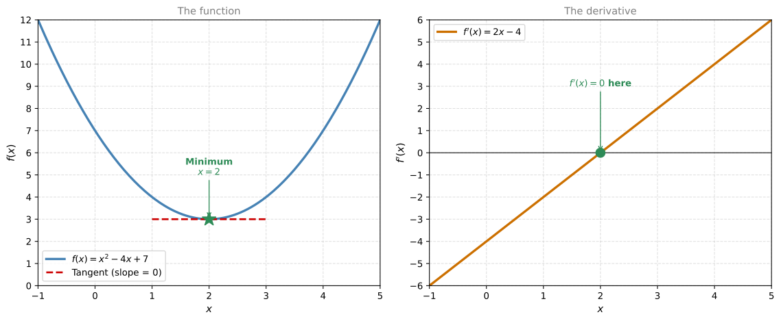
The left plot below shows the function with a flat tangent at the minimum. The right plot shows the derivative, which crosses zero exactly at \(x = 2\).
Using Gradient Descent
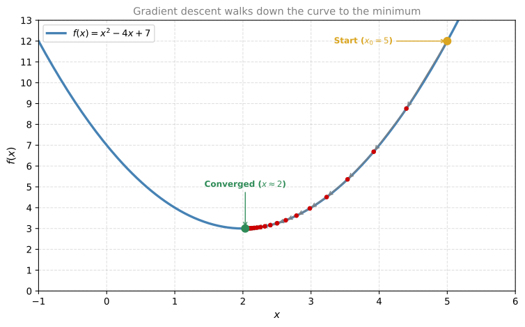
Start at \(x_0 = 5\) with learning rate \(\alpha = 0.1\). The update rule is \(x_{k+1} = x_k - \alpha \cdot f'(x_k) = x_k - 0.1(2x_k - 4)\).
Iteration 1: \[x_1 = 5 - 0.1(2 \cdot 5 - 4) = 5 - 0.6 = 4.4\]
Iteration 2: \[x_2 = 4.4 - 0.1(2 \cdot 4.4 - 4) = 4.4 - 0.48 = 3.92\]
Iteration 3: \[x_3 = 3.92 - 0.1(2 \cdot 3.92 - 4) = 3.92 - 0.384 = 3.536\]
Each step brings us closer to \(x = 2\). After about 20 iterations, \(x_k \approx 2.000\).
Takeaway
Both methods find the same minimum. The derivative approach solves one equation. Gradient descent evaluates the derivative repeatedly and steps downhill. They give the same answer, but gradient descent does not require you to solve anything. You only need to be able to evaluate \(f'(x)\) at each point. This makes it powerful for functions where solving \(f'(x) = 0\) is difficult or impossible.
Power Lines Problem Revisited
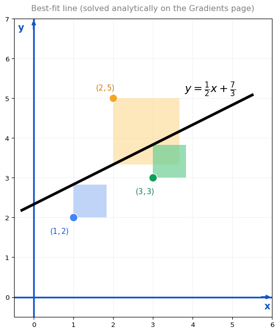
Recall the setup from the Gradients page. Three power lines are at positions \((1, 2)\), \((2, 5)\), and \((3, 3)\). A fiber line \(y = mx + b\) must minimize the total squared connection cost:
\[ E(m, b) = (m + b - 2)^2 + (2m + b - 5)^2 + (3m + b - 3)^2 \]
Analytically, we found the best-fit line \(y = \frac{1}{2}x + \frac{7}{3}\), with minimum cost \(E = 4.167\).
With gradient descent, we do not need to solve any system of equations. We just need the gradient:
\[ \nabla E = \begin{bmatrix} \frac{\partial E}{\partial m} \\\\ \frac{\partial E}{\partial b} \end{bmatrix} = \begin{bmatrix} 28m + 12b - 42 \\\\ 12m + 6b - 20 \end{bmatrix} \]
Then we start at some random point \((m_0, b_0)\) and iterate:
\[ \begin{bmatrix} m_{k+1} \\ b_{k+1} \end{bmatrix} = \begin{bmatrix} m_k \\ b_k \end{bmatrix} - \alpha \cdot \nabla E(m_k, b_k) \]
After enough steps, we arrive at the minimum.
Connecting the Two Plots
There is a nice way to visualize what gradient descent does for linear regression.
On the left, you see the data points and the current line \(y = mx + b\). On the right, you see the cost surface, where each point on the “floor” corresponds to a pair \((m, b)\) and the height is the error \(E(m, b)\).
- A good line (small error) sits near the bottom of the cost surface.
- A bad line (large error) sits high up on the cost surface.
As gradient descent moves down the cost surface, the line fit improves. The interactive tool below animates the process step by step.
Formal Gradient Descent Algorithm for Linear Regression
Now let us write the same idea in its most general form. Instead of 3 power lines, imagine you have \(n\) data points \((x_1, y_1), (x_2, y_2), \ldots, (x_n, y_n)\), and you want to find the line \(y = mx_N + b_N\) that best fits them. This is the same update rule you have been using, just written for any number of points.
The loss function measures how far the line is from all the data points:
\[ \mathscr{L}(m, b) = \frac{1}{2n} \left[ (mx_1 + b - y_1)^2 + \cdots + (mx_n + b - y_n)^2 \right] \]
The gradient descent update rule iterates from step \(N-1\) to step \(N\):
\[ \begin{bmatrix} m_N \\ b_N \end{bmatrix} = \begin{bmatrix} m_{N-1} \\ b_{N-1} \end{bmatrix} - \alpha \, \nabla \mathscr{L}(m_{N-1}, b_{N-1}) \]
where the gradient is:
\[ \nabla \mathscr{L} = \begin{bmatrix} \frac{1}{n} \sum_{i=1}^{n} (mx_i + b - y_i) \cdot x_i \\\\ \frac{1}{n} \sum_{i=1}^{n} (mx_i + b - y_i) \end{bmatrix} \]
The algorithm:
- Start with some random \((m_0, b_0)\). This gives a random line that probably does not fit the data well.
- Compute the gradient \(\nabla \mathscr{L}(m_0, b_0)\).
- Update to get \((m_1, b_1)\), which gives a slightly better line.
- Repeat \(N\) times until the line fits well (that is, until the steps become negligibly small).
Note
This is exactly how linear regression is trained in machine learning. Instead of solving a system of equations (which is expensive for millions of parameters), you iterate the gradient descent formula. It scales to any number of data points and any number of parameters.
Review Questions
1. About the Gradient Descent method, choose all that are true.
- It always converges to a local minimum.
- The result may vary depending on the initial point.
- If it converges, then it converges to a global minimum.
- It only works for differentiable functions.
TipAnswer
b and d.
- b is correct because if the function has several minima, the initial point will dictate to where the algorithm converges.
- d is correct because gradient descent uses the gradient as its base, and the gradient is related to partial derivatives, so we must have differentiable functions to perform the algorithm.
- a is wrong because with a bad learning rate, the algorithm may diverge and never converge.
- c is wrong because gradient descent can get stuck in a local minimum that is not the global minimum.
1. Let \(f(x, y) = 2x^2 + 3y^2 - 2xy - 10x\). The minimum value of \(f(x, y)\) is:
- \(-15\)
- \(3\)
- \(1\)
TipAnswer
a. \(-15\)
1. What are the parameters that the Gradient Descent algorithm has? (check all that apply)
- Initial point
- Final point
- Learning rate
- Number of iterations
TipAnswer
a, c, and d.
- a is correct because the gradient descent algorithm needs an initial point to start its path through the minimum.
- c is correct because the learning rate is the size of each step.
- d is correct because the number of iterations tells us how many times we will perform the calculations. Higher number of iterations will lead to more precise results but will take longer to perform the computations.
- b is wrong because the final point is what we are trying to find, not a parameter we choose.
1. Let \(f(x, y) = x^2 + y^2 - 6x\) and \(\nabla f(x, y) = \begin{bmatrix} 2x - 6 \\ 2y \end{bmatrix}\). Let the initial point be \(x_0 = (0, 1)\). Performing gradient descent with learning rate \(= 0.1\), the first iteration will lead us to the point \(x_1\) which is:
- \(x_1 = (0.6, 0.8)\)
- \(x_1 = (-6, 2)\)
- \(x_1 = (6, -1)\)
- \(x_1 = (0, 1)\)
TipAnswer
a. \(x_1 = (0.6, 0.8)\)
The gradient at \((0, 1)\) is \(\begin{bmatrix} 2(0) - 6 \\ 2(1) \end{bmatrix} = \begin{bmatrix} -6 \\ 2 \end{bmatrix}\).
The update is \(x_1 = (0, 1) - 0.1 \cdot (-6, 2) = (0 + 0.6,\; 1 - 0.2) = (0.6, 0.8)\).