Derivatives and Their Intuition
calculus
Before jumping into the mathematics, let’s understand why calculus is so important in machine learning. The short answer: derivatives are used to…
Why Calculus Matters in Machine Learning
Before jumping into the mathematics, let’s understand why calculus is so important in machine learning. The short answer: derivatives are used to optimize functions, which means finding the maximum or minimum value of a function. When you want to find the model that fits your data in the best possible way, you calculate a loss function and minimize it. Derivatives tell you exactly how to do that.
Example 1: Predicting Sales from TV Advertising (Linear Regression)
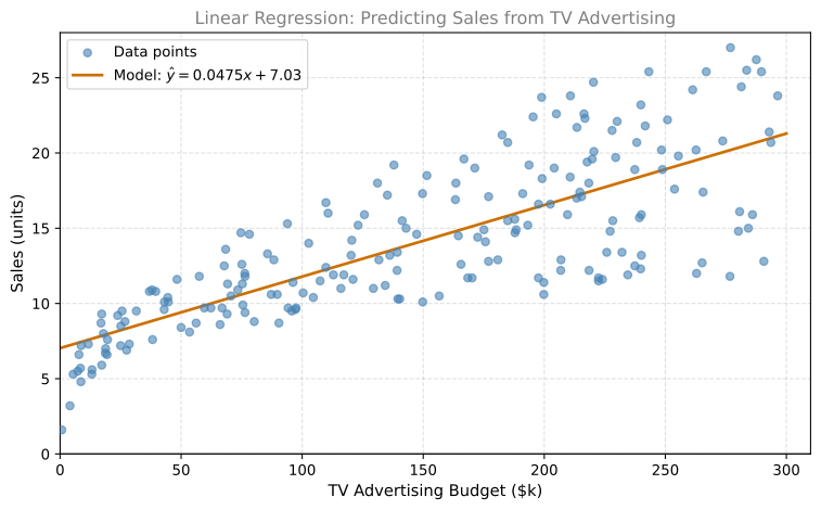
Imagine you work at a company and you have data on how much money was spent on TV advertising and how many units were sold. You want to predict future sales based on the advertising budget. Here are a few rows from the dataset (the full dataset is available on Kaggle or you can download it here):
| TV Advertising Budget ($k) | Sales (units) |
|---|---|
| 230.1 | 22.1 |
| 44.5 | 10.4 |
| 17.2 | 9.3 |
| 151.5 | 18.5 |
| 180.8 | 12.9 |
You decide to build a machine learning model to predict sales. A model, in this case, is simply a line that passes as close as possible to all the data points. The model has parameters (a slope \(w\) and an intercept \(b\)) and predicts \(\hat{y} = wx + b\). When training begins, the model starts with any random line, then tweaks it to get a better fit.
This is called a linear regression problem. But how does the model know which line is best? It defines a loss function that measures how far the predictions are from the actual sales numbers, and then it minimizes that loss. Derivatives are the tool that tell us which direction to adjust \(w\) and \(b\) to make the loss smaller. By computing the derivative of the loss with respect to each parameter, we know exactly how to tweak the model to improve it.
You will see the full details of this process in later pages. Specifically, in Optimization in Neural Networks we build this up from the perceptron all the way to gradient descent on the loss function.
Example 2: Classifying Alien Moods (Classification)
Now consider a different problem. Suppose you travel to a distant planet and meet some aliens. You observe:
| Sentence | “aack” count | “beep” count | Mood |
|---|---|---|---|
| aack aack aack | 3 | 0 | Happy |
| beep beep | 0 | 2 | Sad |
| aack beep aack | 2 | 1 | Happy |
| aack beep beep beep | 1 | 3 | Sad |
You want to tell if an alien is happy or sad based on the sentence. If you plot each sentence as a point (x = number of “aack”, y = number of “beep”), you notice that happy and sad points cluster in different regions. The model here is a line that separates the happy region from the sad region. Training that line requires, once again, derivatives.
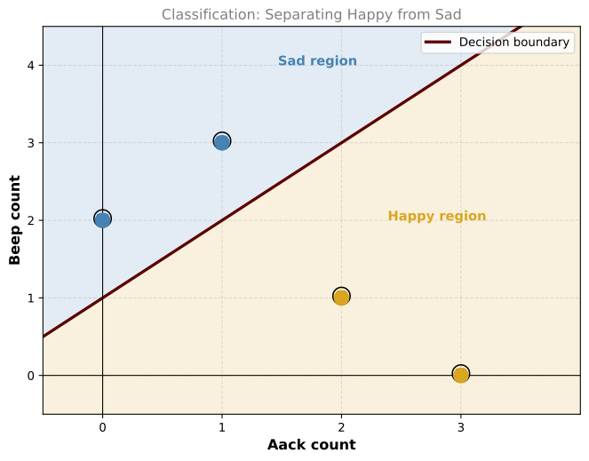
This is called a classification problem. Specifically, since you are classifying mood (happy or sad), it is a sentiment analysis model.
Common Thread
Both problems (and many others in machine learning, including neural networks) rely on the same mathematical machinery:
- Loss/cost functions that measure how far off your model is
- Derivatives that tell you which direction to adjust the model
- Optimization (gradient descent) that iteratively improves the model
In this course, you will learn about derivatives, optimization, and how they power model training.
Derivative as Instantaneous Rate of Change
When you think of a derivative, think of velocity. If you drive 100 km in one hour, your average velocity is 100 km/h. But maybe you started fast, then slowed down, stopped at a light, sped up again, and even reversed at some point. Your velocity was not constant. The question is: at a given instant, what was your velocity?
That is called the instantaneous velocity, and it is precisely what a derivative is. A derivative is the instantaneous rate of change of a function. In this case, the function is distance and its derivative is velocity.
Speedometer Example
Let’s add numbers to this idea. Imagine you are driving on a straight road. You have a speedometer, but it breaks. Fortunately, you have an app that records the distance you have traveled, and you take measurements every 5 seconds for one minute.
| Time (s) | Distance (m) |
|---|---|
| 0 | 0 |
| 5 | 36 |
| 10 | 122 |
| 15 | 202 |
| 20 | 265 |
| 25 | 351 |
| 30 | 441 |
| 35 | 551 |
| 40 | 591 |
| 45 | 716 |
| 50 | 816 |
| 55 | 900 |
| 60 | 1000 |
Is the car moving at constant speed?
Look at the distance values. Between 10 and 15 seconds (a 5-second interval), the car traveled \(202 - 122 = 80\) meters. Between 15 and 20 seconds (also 5 seconds), the car traveled \(265 - 202 = 63\) meters. Since the car covered different distances in equal time intervals, it was not moving at constant speed.
Can we find the velocity at exactly \(t = 12.5\) seconds?
Not exactly. With only data every 5 seconds, we can find the average velocity in an interval, but not the exact velocity at a specific instant within that interval. At \(t = 12.5\), the car might have been going faster or slower than the interval average.
However, we can compute the average velocity between \(t = 10\) and \(t = 15\).
Average Velocity as Slope
The average velocity over an interval is the same as the slope of the line connecting two points on a distance-time graph.
\[ \text{Average velocity} = \frac{\text{change in distance}}{\text{change in time}} = \frac{\Delta d}{\Delta t} \]
This is the “rise over run” formula for slope. For the interval from \(t = 10\) to \(t = 15\):
\[ v_{\text{avg}} = \frac{202 - 122}{15 - 10} = \frac{80}{5} = 16 \text{ m/s} \]
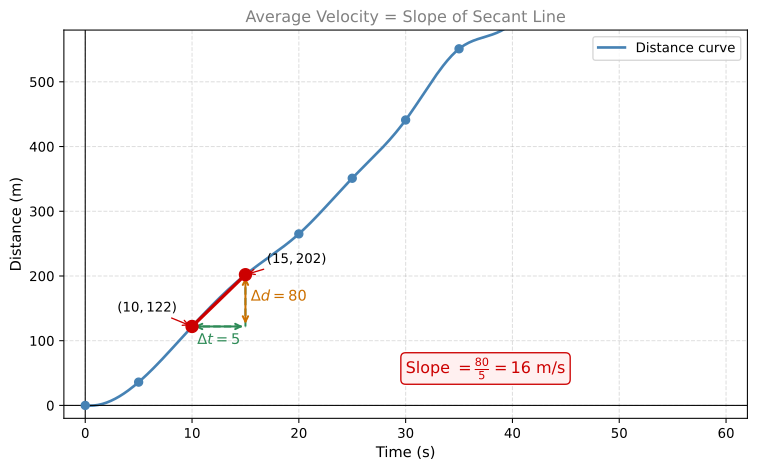
The slope of the line joining \((10, 122)\) and \((15, 202)\) is 16, which means the average velocity between those two points is 16 m/s.
Getting a Better Estimate: Finer Intervals
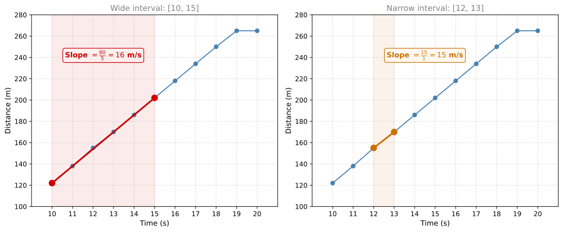
While 16 m/s is a reasonable estimate for the velocity at \(t = 12.5\) seconds, we can do better if we have more data. Suppose we take measurements every 1 second instead of every 5 seconds:
| Time (s) | Distance (m) |
|---|---|
| 10 | 122 |
| 11 | 138 |
| 12 | 155 |
| 13 | 170 |
| 14 | 186 |
| 15 | 202 |
| 16 | 218 |
| 17 | 234 |
| 18 | 250 |
| 19 | 265 |
| 20 | 265 |
Now we can compute the average velocity over the smaller interval from \(t = 12\) to \(t = 13\):
\[ v_{\text{avg}} = \frac{170 - 155}{13 - 12} = \frac{15}{1} = 15 \text{ m/s} \]
This is a much better estimate for the instantaneous velocity at \(t = 12.5\) than the 16 m/s we computed over the 5-second window.
From Average Velocity to the Derivative
Notice the pattern. We still do not have the exact velocity at \(t = 12.5\). But the finer the interval we use, the better our estimate becomes. If we could shrink the interval to be infinitely small, we would get the exact instantaneous velocity. That process of shrinking the interval to zero is exactly what a derivative is. You will see the formal definition soon.
Derivative as a Tangent Line
Let’s revisit the point \(t = 12.5\). Calculating the exact instantaneous velocity here is hard, but we can estimate it by picking a second point to the right and computing the slope of the line joining them. That line is called a secant line.
Now imagine moving that second point closer and closer to \(t = 12.5\). Each time, the secant line tilts slightly, and the slope changes. When the second point gets infinitely close, the secant line becomes the tangent line at \(t = 12.5\). The slope of that tangent line is the derivative.
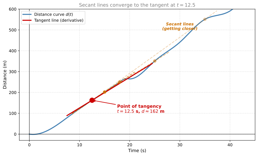
In notation: imagine a tiny change in distance \(dx\) happening over a tiny interval \(dt\). The ratio \(\frac{dx}{dt}\) is the instantaneous rate of change, which is the derivative.
Note
The derivative of a function at a point is precisely the slope of the tangent line at that point.
Slopes, Maxima and Minima
Let’s go back to the 1-second data table. Notice that at \(t = 19\) the distance is 265 m, and at \(t = 20\) the distance is also 265 m. The car did not move in that interval. The line connecting those two points is horizontal, and a horizontal line has a slope of zero:
\[ \text{slope} = \frac{265 - 265}{20 - 19} = \frac{0}{1} = 0 \text{ m/s} \]
Now consider a more general trajectory where a car goes forward, stops, goes backward, stops again, and so on. At what points is the velocity zero? Exactly at the points where the tangent line is horizontal (slope = 0). These are the points where the car momentarily stops.
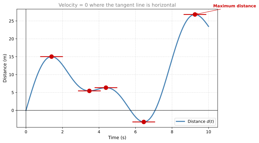
Here is the key insight: the maximum (or minimum) of a function occurs at a point where the derivative is zero. Why? Because if the car is still moving (derivative is not zero), it could go further. Only when it stops (derivative equals zero) can it be at its farthest point.
This fact is enormously useful. If you want to find the maximum or minimum value of a function, look for the points where the derivative equals zero. In machine learning, this is exactly how we minimize loss functions: find where the derivative is zero.
Review Questions
1. What is the derivative of a function, in your own words?
TipAnswer
The derivative is the instantaneous rate of change of a function at a specific point. Geometrically, it is the slope of the tangent line to the curve at that point. In the velocity example, the derivative of the distance function gives you the exact speed at any instant.
1. A car travels 200 meters between \(t = 5\) s and \(t = 10\) s. What is its average velocity over that interval?
TipAnswer
Average velocity \(= \frac{200}{10 - 5} = \frac{200}{5} = 40\) m/s.
1. Why can’t we determine the exact velocity at \(t = 7\) s from only knowing the distances at \(t = 5\) and \(t = 10\)?
TipAnswer
Because we only know what happened at the endpoints of the interval, not what happened in between. The car could have been speeding up, slowing down, or even stopped momentarily at \(t = 7\). All we can compute is the average over the full 5-second window.
1. Why does the maximum or minimum of a function occur where the derivative is zero?
TipAnswer
If the function is still increasing or decreasing (derivative not zero), it has not yet reached its highest or lowest point. Only when the function momentarily stops changing (derivative equals zero, tangent is horizontal) can it be at a maximum or minimum.
1. How does calculus help in machine learning?
TipAnswer
Machine learning models are trained by minimizing a loss function that measures how far off the model’s predictions are. Derivatives (and gradients, their multi-variable generalization) tell the training algorithm which direction to adjust the model parameters to reduce the loss. This iterative process is called gradient descent.