MLE and Linear Regression
statistics
In the previous section, you learned MLE for estimating parameters of Bernoulli and Gaussian distributions. Now we will see how MLE connects to…
In the previous section, you learned MLE for estimating parameters of Bernoulli and Gaussian distributions. Now we will see how MLE connects to something very familiar: linear regression. The key insight is that fitting a line to data using least squares is exactly the same as finding the line that maximizes the likelihood of the data under a Gaussian noise model.
How a Line Generates Points
Imagine a line as a road. If you build houses along that road, the houses are likely to be built close to the road, not far from it. The same idea applies to data points and a regression line.
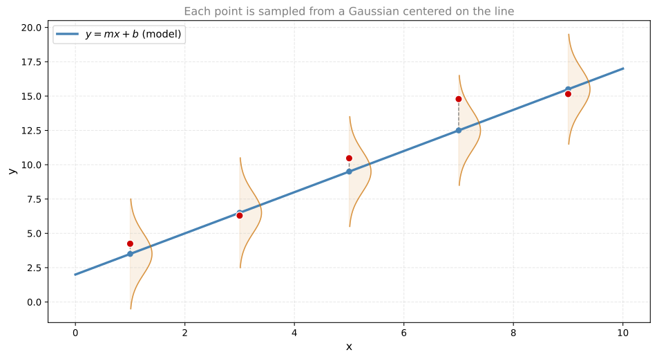
Here is the model: for each value of \(x\), the line gives a predicted value \(y = mx + b\). This predicted value is where the line intersects that vertical position (the blue dots in the plot below). But real data is noisy, so the actual observed value will not land exactly on the line. Instead, we imagine placing a vertical Gaussian (bell curve) centered at the blue dot, and the actual observation (the red dot) is randomly sampled from that Gaussian.
Points that land close to the line are very likely (they are near the center of the Gaussian where probability is high). Points that land far from the line are unlikely (they are in the tails of the Gaussian where probability is low).
The gray dashed lines show the distance \(d_i\) between each red dot (observation) and its corresponding blue dot (prediction on the line). Shorter distances mean higher likelihood.
The orange curves are the Gaussians at each \(x\) position. The blue dots are where the line predicts \(y\) (the center of each Gaussian). The red dots are the actual observed points (randomly sampled from those Gaussians). The gray dashed lines show the distances \(d_i\) between observed and predicted values. A point close to the line was very likely to be generated; a point far from the line was unlikely.
Likelihood of the Data
Given a line \(y = mx + b\) and observed points \((x_1, y_1), \ldots, (x_n, y_n)\), the distance from each point to the line is:
\[ d_i = y_i - (mx_i + b) \]
If we assume each point is generated from a Gaussian with standard deviation \(\sigma\) centered on the line, then the likelihood of generating point \(i\) is:
\[ L_i = \frac{1}{\sqrt{2\pi}\,\sigma} \, e^{-\frac{1}{2}\frac{d_i^2}{\sigma^2}} \]
Since the points are generated independently, the total likelihood is the product:
\[ L = L_1 \cdot L_2 \cdots L_n = \prod_{i=1}^n L_i = \prod_{i=1}^n \frac{1}{\sqrt{2\pi}\,\sigma} \, e^{-\frac{1}{2}\frac{d_i^2}{\sigma^2}} \]
From MLE to Least Squares
Now let us maximize this likelihood. The \(\frac{1}{\sqrt{2\pi}\,\sigma}\) terms are constants (they do not depend on \(m\) or \(b\)), so we can ignore them. What remains is:
\[ L \propto e^{-\frac{1}{2\sigma^2}\sum_{i=1}^n d_i^2} \]
Taking the logarithm:
\[ \log L = -\frac{1}{2\sigma^2}\sum_{i=1}^n d_i^2 + \text{const} \]
Maximizing \(\log L\) means making \(-\sum d_i^2\) as large as possible (as close to zero as possible). Since there is a negative sign, maximizing the log-likelihood is the same as minimizing the sum of squared distances:
\[ \text{Maximize } \log L \quad \Longleftrightarrow \quad \text{Minimize } \sum_{i=1}^n d_i^2 = \sum_{i=1}^n \left(y_i - (mx_i + b)\right)^2 \]
This is precisely the least squares error. Linear regression finds the line that minimizes the sum of squared residuals, which is exactly the same as finding the line that maximizes the likelihood under Gaussian noise.
Visual Comparison
Here are three candidate lines with the Gaussians visualized in 3D. The z-axis shows the probability density at each point. The dark curve connecting the likelihood values at the data points shows how well each model fits:
- Orange line: the regression model (\(y = mx + b\)), lying flat on the ground (z=0 plane)
- Blue curves: Gaussian bell curves standing vertically at each data point, centered on the orange line
- Dark connecting curve: connects the height each data point reaches on its Gaussian. This is the likelihood value at each observation. Tall and even = good fit (all points are near the centers of their Gaussians). Low and uneven = bad fit (points fall in the tails).
- Blue dots: the actual data points on the ground plane
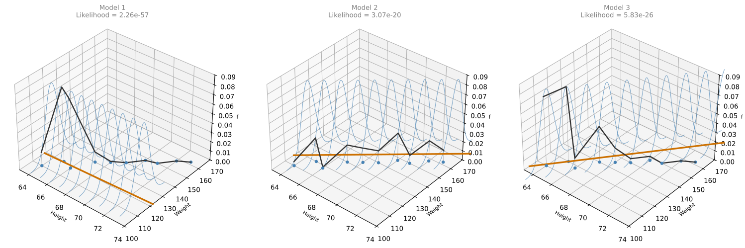
Model 2 has the highest total likelihood because its Gaussians are well-centered on the data points (the red dots are near the peaks of the Gaussians). Models 1 and 3 have the data points landing in the tails of their Gaussians, giving much lower likelihoods.
Key Result
\[ \boxed{\text{MLE with Gaussian noise} \;=\; \text{Linear Regression (Least Squares)}} \]
Finding the line that most likely produced the data using maximum likelihood is exactly the same as minimizing the least squares error. This connection is why linear regression has such a strong theoretical foundation: it is not just a “fit a line” heuristic, it is the maximum likelihood solution under the assumption of Gaussian noise.
Review Questions
1. In the MLE view of linear regression, what role does the Gaussian play?
TipAnswer
The Gaussian models the noise in the data. At each \(x\) value, the observed \(y\) is assumed to be drawn from a Gaussian centered at the line’s prediction (\(mx + b\)). The spread of the Gaussian (\(\sigma\)) represents how noisy the data is.
2. Why does maximizing the likelihood lead to minimizing the sum of squared errors?
TipAnswer
The likelihood is \(\prod e^{-d_i^2/(2\sigma^2)}\), which equals \(e^{-\sum d_i^2/(2\sigma^2)}\). Taking the log gives \(-\sum d_i^2/(2\sigma^2)\). Since this has a negative sign, maximizing it means making \(\sum d_i^2\) as small as possible. That is exactly the least squares criterion.
3. What assumption about the noise makes MLE equivalent to least squares?
TipAnswer
The noise must be Gaussian (normally distributed) with the same variance at every point, and the noise at different points must be independent. If the noise had a different distribution (e.g., heavy tails), MLE would lead to a different loss function, not least squares.
Regularization
So far, MLE picks the model that fits the data best (lowest loss). But fitting too well can be a problem. Consider three models for the same dataset:
- A linear model (\(y = 4x + 3\))
- A quadratic model (\(y = 2x^2 - 4x + 5\))
- A degree-10 polynomial (with many large coefficients)
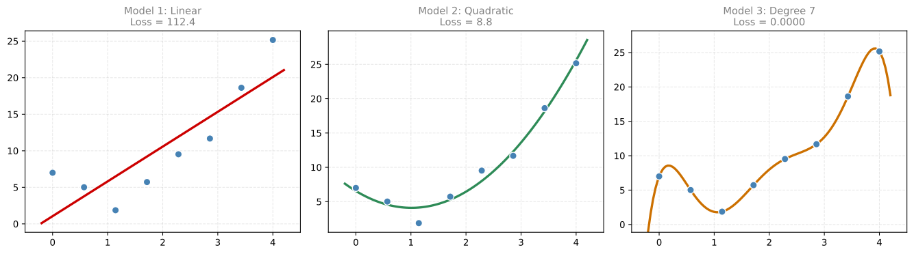
Model 3 has the lowest loss (it passes through almost every point). But it is chaotic and does not generalize well. It memorized the noise rather than learning the underlying pattern. Model 2 captures the true quadratic shape.
Problem: Overfitting
If we only minimize the loss, complex models always win because they can fit the training data perfectly. But they fail on new data. This is called overfitting.
Solution: Penalize Complexity
The idea of regularization is to add a penalty to the loss that grows with model complexity. The more complicated the model (larger coefficients), the higher the penalty.
For a polynomial \(y = a_k x^k + a_{k-1} x^{k-1} + \cdots + a_1 x + a_0\), the \(L_2\) penalty is the sum of the squares of all coefficients (except the constant \(a_0\)):
\[ L_2 \text{ penalty} = a_1^2 + a_2^2 + \cdots + a_k^2 \]
Worked Example
| Model | Equation | Loss | \(L_2\) Penalty | Regularized Loss |
|---|---|---|---|---|
| 1 | \(y = 4x + 3\) | 10 | \(4^2 = 16\) | \(10 + 16 = 26\) |
| 2 | \(y = 2x^2 - 4x + 5\) | 2 | \(2^2 + (-4)^2 = 20\) | \(2 + 20 = 22\) ← winner |
| 3 | \(y = 4x^{10} - 9x^8 - 2x^6 + 3x^5 - 6x^4 - 10x + 4\) | 0.1 | \(4^2 + 9^2 + 2^2 + 3^2 + 6^2 + 10^2 = 246\) | \(0.1 + 246 = 246.1\) |
Without regularization, Model 3 wins (loss = 0.1). With regularization, Model 2 wins (regularized loss = 22). The penalty discourages the chaotic model with huge coefficients.
Regularization Term
In general, suppose our model is a polynomial:
\[ y = a_n x^n + a_{n-1} x^{n-1} + \cdots + a_1 x + a_0 \]
The coefficients \(a_n, a_{n-1}, \ldots, a_1\) (all except the constant \(a_0\)) are the ones we penalize. Large coefficients mean the model is complex and wiggly. The constant \(a_0\) just shifts the curve up or down, so it does not contribute to complexity.
Log-loss: \(\ell\ell\) (the original loss, such as sum of squared errors)
\(L_2\) Regularization Error: the sum of the squares of all coefficients except the constant:
\[ a_n^2 + a_{n-1}^2 + \cdots + a_1^2 \]
Regularization parameter: \(\lambda\) (a number you choose that controls how much to penalize complexity)
Regularized error: the total cost you minimize is the log-loss plus \(\lambda\) times the penalty:
\[ \text{Regularized error} = \ell\ell + \lambda\left(a_n^2 + a_{n-1}^2 + \cdots + a_1^2\right) \]
When \(\lambda\) is small, the penalty barely matters and you mostly minimize the loss (risk of overfitting). When \(\lambda\) is large, the penalty dominates and forces the coefficients to be small, producing a simpler model (risk of underfitting). Choosing the right \(\lambda\) is a balancing act.
Review Questions
4. Why does minimizing loss alone sometimes lead to overfitting?
TipAnswer
Because complex models (high-degree polynomials) have enough flexibility to pass through every data point, achieving near-zero loss on the training data. But they are fitting the noise, not the underlying pattern, so they perform poorly on new data.
5. What does the \(L_2\) penalty measure?
TipAnswer
The sum of the squares of the model coefficients (excluding the constant). Large coefficients mean the model is complex and potentially overfitting. The \(L_2\) penalty is large when coefficients are large, discouraging overly complex models.
6. If \(\lambda = 0\), what happens to the regularized error?
TipAnswer
The regularized error becomes just the loss (no penalty). This is equivalent to standard MLE with no regularization, which may lead to overfitting if the model is complex enough.
7. How do you account for penalty and loss values when determining the best model with regularization?
- Calculate the new loss as the sum of the penalty and the previous loss.
- Set the new loss equal to the penalty value.
TipAnswer
a. When incorporating regularization into the loss function, the penalty term is added to the previous loss to form the new loss. This ensures that the penalty for complexity is appropriately balanced with the original loss.
8. Why is regularization important in machine learning?
- To increase the complexity of the model.
- To prevent overfitting and improve generalization.
- To introduce randomness into the model.
TipAnswer
b. Regularization techniques help prevent overfitting by adding a penalty term to the loss function, which discourages overly complex models. This improves the model’s ability to generalize well to unseen data.
9. Suppose you flip a coin 10 times and obtain 6 heads and 4 tails. What function needs to be maximized to find the MLE of \(p\)?
- \(L(p) = p^{1/6}(1-p)^{1/4}\)
- \(L(p) = p^6(1-p)^4\)
- \(L(p) = p^4(1-p)^6\)
- \(L(p) = p^{10}(1-p)^0\)
TipAnswer
b. The likelihood for \(k\) heads and \(n-k\) tails is \(L(p) = p^k(1-p)^{n-k}\). With 6 heads and 4 tails: \(L(p) = p^6(1-p)^4\).
10. Which of the following statements about linear regression is true?
- Linear regression minimizes the sum of squared distances between the points and the fitted line, providing the best fit to the data.
- Linear regression connects two random points in the dataset to fit the data.
- Linear regression aims to maximize the sum of squared distances between the points and the fitted line.
- Linear regression is unrelated to finding the best fit line for a given dataset.
TipAnswer
a. Linear regression finds the line that minimizes \(\sum(y_i - (mx_i + b))^2\), the sum of squared vertical distances from the data points to the line. This is equivalent to MLE under Gaussian noise.
11. What is the purpose of regularization in machine learning?
- Regularization favors more complex models to increase performance on the training data.
- Regularization prevents overfitting by penalizing models with large coefficients or weights.
- Regularization is used to increase the training error of a model, which can improve its generalization performance.
- Regularization is used to improve the interpretability of a model by reducing its complexity.
TipAnswer
b. Regularization adds a penalty term (like \(\lambda \sum a_j^2\)) to the loss function that grows with the size of the coefficients. This discourages overly complex models and helps the model generalize better to unseen data.
12. A model \(M = 4x^4 + 3x^2 + 1\) best fits the data. What is the \(L_2\) regularization error value for this model?
- 8
- 25
- 26
- 144
TipAnswer
b. The \(L_2\) regularization error is the sum of squared coefficients (excluding the constant): \(4^2 + 3^2 = 16 + 9 = 25\). The constant term (1) is not included in the penalty.