import pandas as pd
import seaborn as snsLab: Intro to Pandas
probability
Welcome to the Pandas tutorial lab. This is the first notebook of the exploratory data analysis (EDA) series, where you will get hands-on practice…
Welcome to the Pandas tutorial lab. This is the first notebook of the exploratory data analysis (EDA) series, where you will get hands-on practice applying skills from the course to a real data problem. Here you will see and try out some basics of Pandas and get familiar with useful functions that you will use across other labs and assignments.
For demonstration purposes, you will use the World Happiness Report dataset. The dataset consists of 2199 rows, where each row contains various happiness-related metrics for a certain country in a given year. You will use this dataset to understand some fundamental operations in Pandas.
Download the dataset: world_happiness.csv
Importing Libraries
The most important library you will need is Pandas. You will also use the Seaborn library for plotting. To import them, run the cell below.
Loading Data
Now that you have the Pandas library imported, you need to load your dataset. The dataset is saved as a .csv file and you can load it by calling pd.read_csv(filename). When you load the dataset, it will be stored as a DataFrame type. This is the most commonly used Pandas data structure that you will use throughout this and other notebooks.
df = pd.read_csv('../../media/world_happiness.csv')Basic Operations
Viewing Data with head() and tail()
You can use df.head() and df.tail() to view the first or last rows of the DataFrame respectively. By default, these show five rows, but you can specify the number of rows as a parameter.
df.head()| Country name | year | Life Ladder | Log GDP per capita | Social support | Healthy life expectancy at birth | Freedom to make life choices | Generosity | Perceptions of corruption | Positive affect | Negative affect | |
|---|---|---|---|---|---|---|---|---|---|---|---|
| 0 | Afghanistan | 2008 | 3.724 | 7.350 | 0.451 | 50.5 | 0.718 | 0.168 | 0.882 | 0.414 | 0.258 |
| 1 | Afghanistan | 2009 | 4.402 | 7.509 | 0.552 | 50.8 | 0.679 | 0.191 | 0.850 | 0.481 | 0.237 |
| 2 | Afghanistan | 2010 | 4.758 | 7.614 | 0.539 | 51.1 | 0.600 | 0.121 | 0.707 | 0.517 | 0.275 |
| 3 | Afghanistan | 2011 | 3.832 | 7.581 | 0.521 | 51.4 | 0.496 | 0.164 | 0.731 | 0.480 | 0.267 |
| 4 | Afghanistan | 2012 | 3.783 | 7.661 | 0.521 | 51.7 | 0.531 | 0.238 | 0.776 | 0.614 | 0.268 |
df.tail(2)| Country name | year | Life Ladder | Log GDP per capita | Social support | Healthy life expectancy at birth | Freedom to make life choices | Generosity | Perceptions of corruption | Positive affect | Negative affect | |
|---|---|---|---|---|---|---|---|---|---|---|---|
| 2197 | Zimbabwe | 2021 | 3.155 | 7.657 | 0.685 | 54.050 | 0.668 | -0.076 | 0.757 | 0.610 | 0.242 |
| 2198 | Zimbabwe | 2022 | 3.296 | 7.670 | 0.666 | 54.525 | 0.652 | -0.070 | 0.753 | 0.641 | 0.191 |
Index and Columns
In a DataFrame, data is stored in a two-dimensional grid (rows and columns). The rows are indexed and the columns are named. You can inspect these with df.index and df.columns.
df.indexRangeIndex(start=0, stop=2199, step=1)As you can see, the index is a range of numbers between 0 (inclusive) and 2199 (not inclusive). Now look at the column names.
df.columnsIndex(['Country name', 'year', 'Life Ladder', 'Log GDP per capita',
'Social support', 'Healthy life expectancy at birth',
'Freedom to make life choices', 'Generosity',
'Perceptions of corruption', 'Positive affect', 'Negative affect'],
dtype='str')The column names contain spaces, which can cause difficulties when accessing them. A common practice is to replace spaces with underscores and make everything lowercase. You can rename columns using df.rename() with a dictionary mapping old names to new names.
# Build a dictionary mapping old column names to new ones (lowercase, underscores for spaces)
columns_to_rename = {i: "_".join(i.split(" ")).lower() for i in df.columns}

# Rename the columns
df = df.rename(columns=columns_to_rename)
df.head()| country_name | year | life_ladder | log_gdp_per_capita | social_support | healthy_life_expectancy_at_birth | freedom_to_make_life_choices | generosity | perceptions_of_corruption | positive_affect | negative_affect | |
|---|---|---|---|---|---|---|---|---|---|---|---|
| 0 | Afghanistan | 2008 | 3.724 | 7.350 | 0.451 | 50.5 | 0.718 | 0.168 | 0.882 | 0.414 | 0.258 |
| 1 | Afghanistan | 2009 | 4.402 | 7.509 | 0.552 | 50.8 | 0.679 | 0.191 | 0.850 | 0.481 | 0.237 |
| 2 | Afghanistan | 2010 | 4.758 | 7.614 | 0.539 | 51.1 | 0.600 | 0.121 | 0.707 | 0.517 | 0.275 |
| 3 | Afghanistan | 2011 | 3.832 | 7.581 | 0.521 | 51.4 | 0.496 | 0.164 | 0.731 | 0.480 | 0.267 |
| 4 | Afghanistan | 2012 | 3.783 | 7.661 | 0.521 | 51.7 | 0.531 | 0.238 | 0.776 | 0.614 | 0.268 |
Data Types
One powerful feature of DataFrames is that columns can have different data types (dtypes). You can inspect them with df.dtypes.
df.dtypescountry_name str
year int64
life_ladder float64
log_gdp_per_capita float64
social_support float64
healthy_life_expectancy_at_birth float64
freedom_to_make_life_choices float64
generosity float64
perceptions_of_corruption float64
positive_affect float64
negative_affect float64
dtype: objectIf your data has incorrectly formatted types, you can change them manually using df.astype().
# List all columns that should be floats
float_columns = [i for i in df.columns if i not in ["country_name", "year"]]

# Change the type of all float columns to float
df = df.astype({i: float for i in float_columns})
df.dtypes
country_name str
year int64
life_ladder float64
log_gdp_per_capita float64
social_support float64
healthy_life_expectancy_at_birth float64
freedom_to_make_life_choices float64
generosity float64
perceptions_of_corruption float64
positive_affect float64
negative_affect float64
dtype: objectThe df.info() method provides additional information, including the number of non-null values per column.
df.info()<class 'pandas.DataFrame'>
RangeIndex: 2199 entries, 0 to 2198
Data columns (total 11 columns):
# Column Non-Null Count Dtype
--- ------ -------------- -----
0 country_name 2199 non-null str
1 year 2199 non-null int64
2 life_ladder 2199 non-null float64
3 log_gdp_per_capita 2179 non-null float64
4 social_support 2186 non-null float64
5 healthy_life_expectancy_at_birth 2145 non-null float64
6 freedom_to_make_life_choices 2166 non-null float64
7 generosity 2126 non-null float64
8 perceptions_of_corruption 2083 non-null float64
9 positive_affect 2175 non-null float64
10 negative_affect 2183 non-null float64
dtypes: float64(9), int64(1), str(1)
memory usage: 206.8 KBSelecting Columns
One way to select a single column is dot notation: df.column_name. This is why it was a good idea to rename columns without spaces. This returns a Pandas Series.
x = df.life_ladder
print(f"type(x):\n {type(x)}\n")
print(f"x:\n{x}")
type(x):
<class 'pandas.Series'>
x:
0 3.724
1 4.402
2 4.758
3 3.832
4 3.783
...
2194 3.616
2195 2.694
2196 3.160
2197 3.155
2198 3.296
Name: life_ladder, Length: 2199, dtype: float64Another way is to use square brackets with the column name as a string, similar to accessing a dictionary entry.
x = df["life_ladder"]
print(f"type(x):\n {type(x)}\n")
print(f"x:\n{x}")
type(x):
<class 'pandas.Series'>
x:
0 3.724
1 4.402
2 4.758
3 3.832
4 3.783
...
2194 3.616
2195 2.694
2196 3.160
2197 3.155
2198 3.296
Name: life_ladder, Length: 2199, dtype: float64Passing a list of column names selects multiple columns and returns a DataFrame (rather than a Series).
x = df[["life_ladder"]]
print(f"type(x):\n {type(x)}\n")
print(f"x:\n{x}")
type(x):
<class 'pandas.DataFrame'>
x:
life_ladder
0 3.724
1 4.402
2 4.758
3 3.832
4 3.783
... ...
2194 3.616
2195 2.694
2196 3.160
2197 3.155
2198 3.296
[2199 rows x 1 columns]Selecting Rows
Passing a slice selects matching rows and returns a DataFrame with all columns.
df[2:5]| country_name | year | life_ladder | log_gdp_per_capita | social_support | healthy_life_expectancy_at_birth | freedom_to_make_life_choices | generosity | perceptions_of_corruption | positive_affect | negative_affect | |
|---|---|---|---|---|---|---|---|---|---|---|---|
| 2 | Afghanistan | 2010 | 4.758 | 7.614 | 0.539 | 51.1 | 0.600 | 0.121 | 0.707 | 0.517 | 0.275 |
| 3 | Afghanistan | 2011 | 3.832 | 7.581 | 0.521 | 51.4 | 0.496 | 0.164 | 0.731 | 0.480 | 0.267 |
| 4 | Afghanistan | 2012 | 3.783 | 7.661 | 0.521 | 51.7 | 0.531 | 0.238 | 0.776 | 0.614 | 0.268 |
Iterating Over Rows
If you ever need to walk through the DataFrame row by row, you can use the .iterrows() method. For each row it gives you a pair: the index of the row and the row itself as a Series. The cell below uses next() to pull out just the first row.
index, row = next(df.iterrows())
row
country_name Afghanistan
year 2008
life_ladder 3.724
log_gdp_per_capita 7.35
social_support 0.451
healthy_life_expectancy_at_birth 50.5
freedom_to_make_life_choices 0.718
generosity 0.168
perceptions_of_corruption 0.882
positive_affect 0.414
negative_affect 0.258
Name: 0, dtype: objectKeep in mind that looping over rows one at a time is slow for large datasets. Pandas is designed so that most operations (like the column arithmetic you will see later in this lab) work on entire columns at once, so you rarely need an explicit loop.
Boolean Indexing
What if you are interested only in data from a certain year, or where a value in a column is greater than some threshold? You can use boolean indexing.
# Select rows where year equals 2022
df[df["year"] == 2022]| country_name | year | life_ladder | log_gdp_per_capita | social_support | healthy_life_expectancy_at_birth | freedom_to_make_life_choices | generosity | perceptions_of_corruption | positive_affect | negative_affect | |
|---|---|---|---|---|---|---|---|---|---|---|---|
| 13 | Afghanistan | 2022 | 1.281 | NaN | 0.228 | 54.875 | 0.368 | NaN | 0.733 | 0.206 | 0.576 |
| 28 | Albania | 2022 | 5.212 | 9.626 | 0.724 | 69.175 | 0.802 | -0.066 | 0.846 | 0.547 | 0.255 |
| 59 | Argentina | 2022 | 6.261 | 10.011 | 0.893 | 67.250 | 0.825 | -0.128 | 0.810 | 0.724 | 0.284 |
| 75 | Armenia | 2022 | 5.382 | 9.668 | 0.811 | 67.925 | 0.790 | -0.154 | 0.705 | 0.531 | 0.549 |
| 91 | Australia | 2022 | 7.035 | 10.854 | 0.942 | 71.125 | 0.854 | 0.153 | 0.545 | 0.711 | 0.244 |
| ... | ... | ... | ... | ... | ... | ... | ... | ... | ... | ... | ... |
| 2104 | Uruguay | 2022 | 6.671 | 10.084 | 0.905 | 67.500 | 0.878 | -0.052 | 0.631 | 0.775 | 0.267 |
| 2120 | Uzbekistan | 2022 | 6.016 | 8.990 | 0.879 | 65.600 | 0.959 | 0.309 | 0.616 | 0.741 | 0.225 |
| 2137 | Venezuela | 2022 | 5.949 | NaN | 0.899 | 63.875 | 0.770 | NaN | 0.798 | 0.754 | 0.292 |
| 2154 | Vietnam | 2022 | 6.267 | 9.333 | 0.879 | 65.600 | 0.975 | -0.179 | 0.703 | 0.774 | 0.108 |
| 2198 | Zimbabwe | 2022 | 3.296 | 7.670 | 0.666 | 54.525 | 0.652 | -0.070 | 0.753 | 0.641 | 0.191 |
114 rows × 11 columns
After filtering, the index has gaps. You can reset it with reset_index(drop=True) if you want the index to correspond to actual row numbers.
new_df = df[df["year"] == 2022]
new_df = new_df.reset_index(drop=True)
new_df| country_name | year | life_ladder | log_gdp_per_capita | social_support | healthy_life_expectancy_at_birth | freedom_to_make_life_choices | generosity | perceptions_of_corruption | positive_affect | negative_affect | |
|---|---|---|---|---|---|---|---|---|---|---|---|
| 0 | Afghanistan | 2022 | 1.281 | NaN | 0.228 | 54.875 | 0.368 | NaN | 0.733 | 0.206 | 0.576 |
| 1 | Albania | 2022 | 5.212 | 9.626 | 0.724 | 69.175 | 0.802 | -0.066 | 0.846 | 0.547 | 0.255 |
| 2 | Argentina | 2022 | 6.261 | 10.011 | 0.893 | 67.250 | 0.825 | -0.128 | 0.810 | 0.724 | 0.284 |
| 3 | Armenia | 2022 | 5.382 | 9.668 | 0.811 | 67.925 | 0.790 | -0.154 | 0.705 | 0.531 | 0.549 |
| 4 | Australia | 2022 | 7.035 | 10.854 | 0.942 | 71.125 | 0.854 | 0.153 | 0.545 | 0.711 | 0.244 |
| ... | ... | ... | ... | ... | ... | ... | ... | ... | ... | ... | ... |
| 109 | Uruguay | 2022 | 6.671 | 10.084 | 0.905 | 67.500 | 0.878 | -0.052 | 0.631 | 0.775 | 0.267 |
| 110 | Uzbekistan | 2022 | 6.016 | 8.990 | 0.879 | 65.600 | 0.959 | 0.309 | 0.616 | 0.741 | 0.225 |
| 111 | Venezuela | 2022 | 5.949 | NaN | 0.899 | 63.875 | 0.770 | NaN | 0.798 | 0.754 | 0.292 |
| 112 | Vietnam | 2022 | 6.267 | 9.333 | 0.879 | 65.600 | 0.975 | -0.179 | 0.703 | 0.774 | 0.108 |
| 113 | Zimbabwe | 2022 | 3.296 | 7.670 | 0.666 | 54.525 | 0.652 | -0.070 | 0.753 | 0.641 | 0.191 |
114 rows × 11 columns
Summary Statistics
Pandas provides a simple way to calculate summary statistics using describe(). It shows count, mean, standard deviation, min, 25th percentile, 50th percentile (median), 75th percentile, and max for each numeric column.
df.describe()| year | life_ladder | log_gdp_per_capita | social_support | healthy_life_expectancy_at_birth | freedom_to_make_life_choices | generosity | perceptions_of_corruption | positive_affect | negative_affect | |
|---|---|---|---|---|---|---|---|---|---|---|
| count | 2199.000000 | 2199.000000 | 2179.000000 | 2186.000000 | 2145.000000 | 2166.000000 | 2126.000000 | 2083.000000 | 2175.000000 | 2183.000000 |
| mean | 2014.161437 | 5.479227 | 9.389760 | 0.810681 | 63.294582 | 0.747847 | 0.000091 | 0.745208 | 0.652148 | 0.271493 |
| std | 4.718736 | 1.125527 | 1.153402 | 0.120953 | 6.901104 | 0.140137 | 0.161079 | 0.185835 | 0.105913 | 0.086872 |
| min | 2005.000000 | 1.281000 | 5.527000 | 0.228000 | 6.720000 | 0.258000 | -0.338000 | 0.035000 | 0.179000 | 0.083000 |
| 25% | 2010.000000 | 4.647000 | 8.500000 | 0.747000 | 59.120000 | 0.656250 | -0.112000 | 0.688000 | 0.572000 | 0.208000 |
| 50% | 2014.000000 | 5.432000 | 9.499000 | 0.836000 | 65.050000 | 0.770000 | -0.023000 | 0.800000 | 0.663000 | 0.261000 |
| 75% | 2018.000000 | 6.309500 | 10.373500 | 0.905000 | 68.500000 | 0.859000 | 0.092000 | 0.869000 | 0.738000 | 0.323000 |
| max | 2022.000000 | 8.019000 | 11.664000 | 0.987000 | 74.475000 | 0.985000 | 0.703000 | 0.983000 | 0.884000 | 0.705000 |
Keep in mind that not all summary statistics always make sense. You have data for many different countries across different years. Are there the same number of datapoints for each country or year? Countries have vastly different populations, so simply averaging numbers out may not tell the full story.
Plotting
DataFrame.plot()
If you want to plot data, you can use df.plot(). By default it uses the index as the x-axis and plots all numeric columns as y-axes. Run the cell below and look closely at the result before reading on.
df.plot()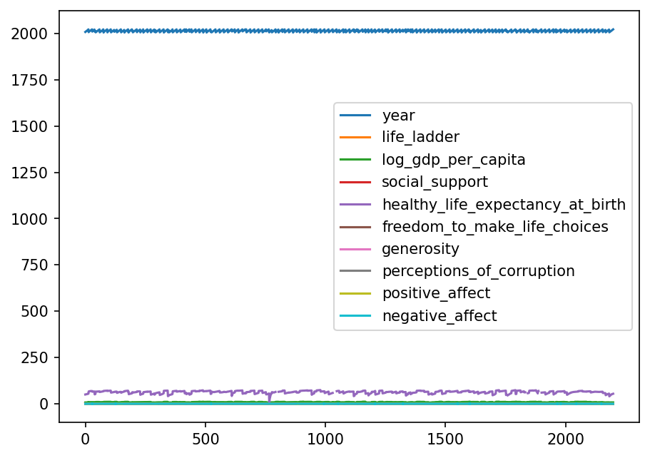
At first glance something seems wrong: the legend lists ten columns, but you can only see about three lines. Where did the rest go?
Look at the y-axis. It has to stretch all the way up to about 2022 to fit the year column, and that choice of scale hides almost everything else:
- The blue band at the top is
year. It looks fuzzy because the years 2005–2022 repeat over and over, once for each country. - The purple line hovering just above zero is
healthy_life_expectancy_at_birth, with values roughly between 7 and 75. - All eight remaining columns (life ladder, log GDP, social support, and so on) have values between about \(-0.3\) and \(12\). On an axis that reaches 2022, that entire range is squeezed into a couple of pixels, so those eight lines are drawn right on top of each other and look like a single flat line at zero.
So the plot is not very useful here: the index has no specific meaning, and the columns live on wildly different scales. But it teaches an important lesson — before plotting everything at once, check whether your columns are even comparable. Try setting some parameters of the .plot() method to see what it allows you to do (for example, logy=True or a list of columns via y=...). You can find all the options in the DataFrame.plot documentation.
Scatter Plots
Pandas can produce genuinely useful plots — you just need to choose the variables yourself. The cell below draws a scatter plot with kind='scatter' and specifically chosen x and y variables. On the x-axis there is the logarithm of GDP per capita (measuring the wealth of a country), and on the y-axis there is the life ladder — an estimate of self-assessed life quality on a scale of 1 to 10, taken from surveys.
df.plot(kind='scatter', x='log_gdp_per_capita', y='life_ladder')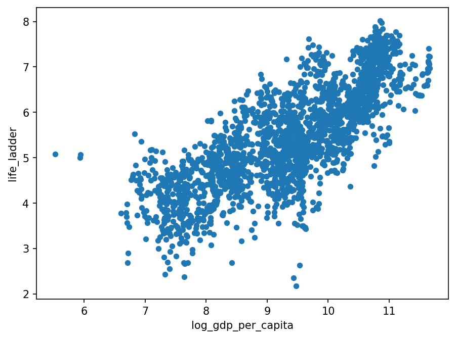
You can see that there is some sort of trend between the wealth of a country and the happiness of its population: wealthier countries tend to have higher life ladder scores. You will explore this kind of relationship much more deeply in later sections on covariance and correlation.
Coloring the Points
Sometimes it is very insightful to color the points to highlight the ones you are most interested in. One way to do this in plain Pandas is to build a color for every row yourself. The cell below creates a dictionary mapping a few chosen countries to colors, then uses a list comprehension to look up the color for each row — cmap.get(c, 'yellow') returns the country’s color if it is in the dictionary, and 'yellow' otherwise.
# Create a dictionary to map the country names to colors
cmap = {
    'Brazil': 'Green',
    'Slovenia': 'Orange',
    'India': 'purple'
}

df.plot(
    kind='scatter',
    x='log_gdp_per_capita',
    y='life_ladder',
    c=[cmap.get(c, 'yellow') for c in df.country_name],  # Set the colors
    s=2  # Set the size of the points
)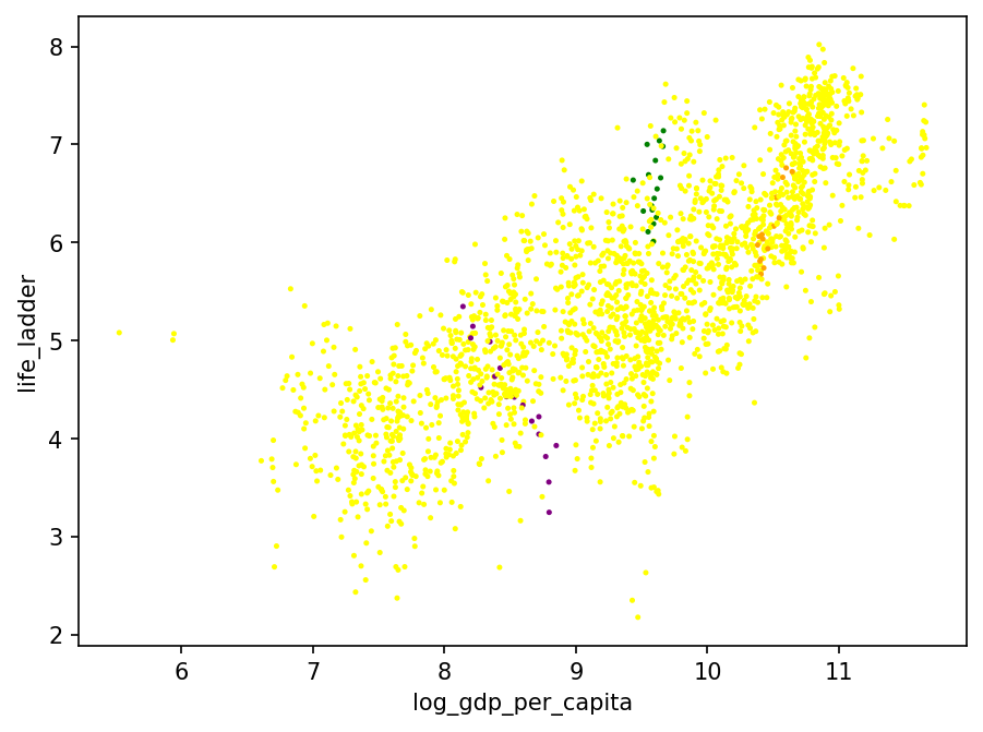
Even though higher GDP generally means a higher value on the life ladder, this is not a universal truth. Compare Slovenia (orange) with Brazil (green): people in Brazil earn less, but through the years they report being on average happier than Slovenians.
Histograms
Another very useful thing you can do with plots is visualize the distribution of your data: which values are common and which are rare. You will study distributions in detail in later sections, but you can already plot a histogram with df.hist(). Note that if you call it on the whole DataFrame, it draws a histogram for every numeric column — so it is often better to name the column you want.
df.hist("life_ladder")array([[<Axes: title={'center': 'life_ladder'}>]], dtype=object)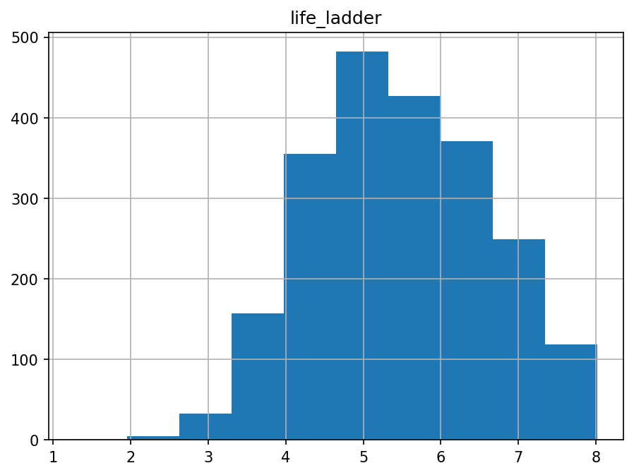
What you see is the distribution of values in the life_ladder column. What do you think about it at first glance — are people generally happy with their quality of life? Be careful before answering: each value here is not a single person’s answer, but an already aggregated score for a whole country in a given year. To answer the question properly, you would need to dig deeper into where each value comes from.
Seaborn Scatterplot
Beyond what Pandas offers, you can use external libraries to easily produce more advanced plots. One such library is Seaborn, which you already imported at the beginning of this lab as sns. Remember the manual color dictionary you built above? Seaborn does the same job in one line with the hue parameter — and it adds a legend automatically. Below, you filter for a few selected countries and color the points by country name.
# Select a few countries of interest
countries = ["Brazil", "Finland", "Japan", "United States", "India"]
df_selected = df[df["country_name"].isin(countries)]

# Create a scatterplot with color by country
sns.scatterplot(data=df_selected, x="log_gdp_per_capita", y="life_ladder", hue="country_name")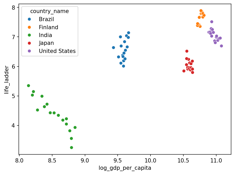
Each country forms its own little cloud: within one country, wealth changes slowly over the years while happiness moves around it. Comparing the clouds shows the same overall trend as before — wealthier countries tend to sit higher on the life ladder.
Pairplot
You can also use sns.pairplot() to visualize pairwise relationships between all numeric variables in the DataFrame. With this kind of plot, you see a scatter plot for each pair of columns. On the diagonal (where a column would be plotted against itself), you get a histogram of that column instead — a scatter plot there would only show a straight line. This can be very useful for initial exploration, though it may take a while with larger datasets.
# The pairplot is a 10x10 grid, so render it at standard dpi to keep the file size down
import matplotlib
matplotlib.rcParams["figure.dpi"] = 96

sns.pairplot(df)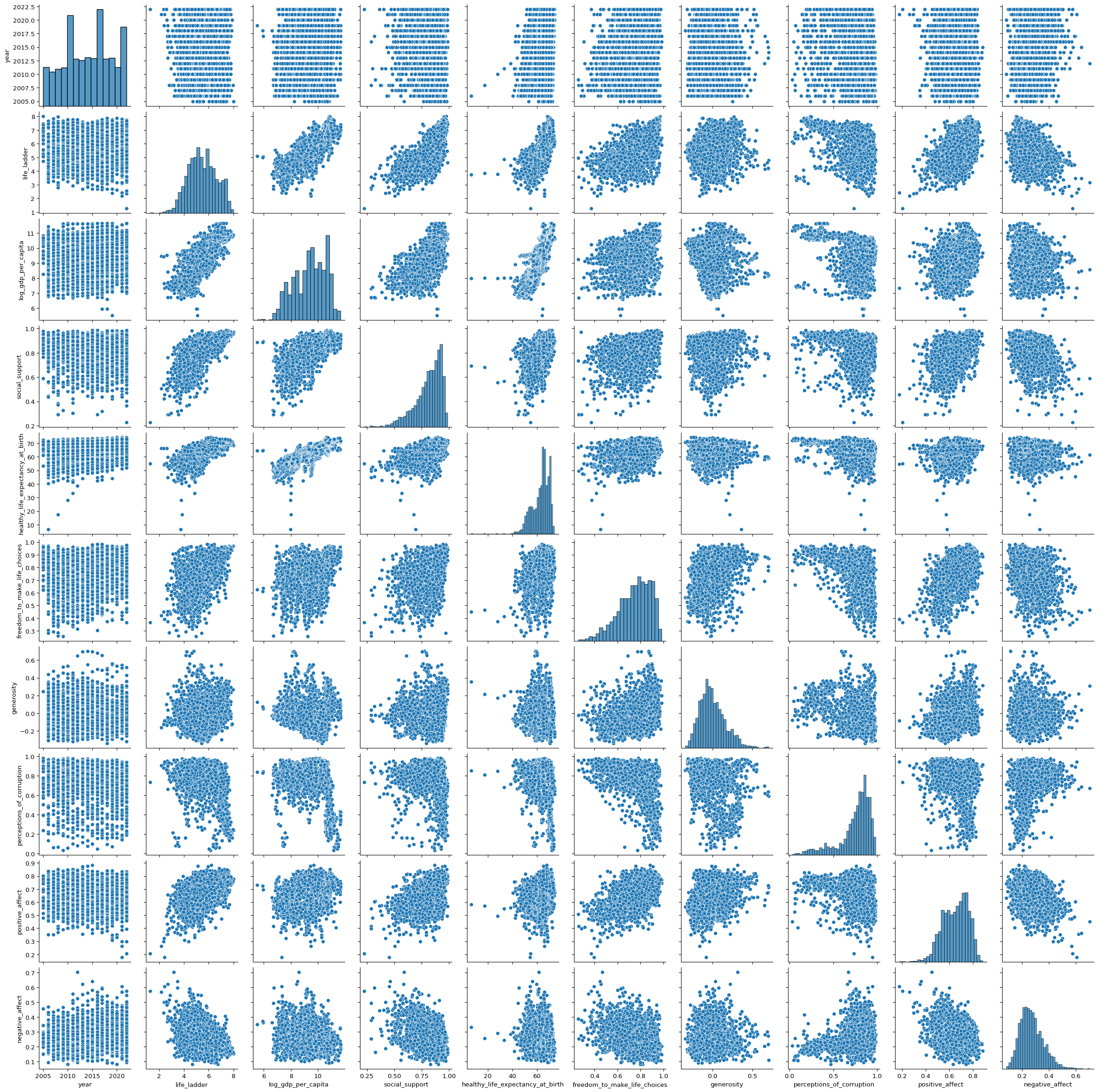
The scatter plots and histograms have very different shapes across columns. Some pairs form elongated clouds (a hint that the two variables may be correlated), others look like shapeless blobs. Think about what insights you could get from this kind of visualization — which pairs of variables would you investigate first?
Operations on Columns
Creating New Columns with Arithmetic
You can create new columns using arithmetic operations on existing columns. This is a powerful tool for feature engineering.
# Create a new column: sum of year and life_ladder (not meaningful, just for demonstration)
df["this_column_makes_no_sense"] = df["year"] + df["life_ladder"]

# Create a new column: difference between positive and negative affect
df["net_affect_difference"] = df["positive_affect"] - df["negative_affect"]

df.head()| country_name | year | life_ladder | log_gdp_per_capita | social_support | healthy_life_expectancy_at_birth | freedom_to_make_life_choices | generosity | perceptions_of_corruption | positive_affect | negative_affect | this_column_makes_no_sense | net_affect_difference | |
|---|---|---|---|---|---|---|---|---|---|---|---|---|---|
| 0 | Afghanistan | 2008 | 3.724 | 7.350 | 0.451 | 50.5 | 0.718 | 0.168 | 0.882 | 0.414 | 0.258 | 2011.724 | 0.156 |
| 1 | Afghanistan | 2009 | 4.402 | 7.509 | 0.552 | 50.8 | 0.679 | 0.191 | 0.850 | 0.481 | 0.237 | 2013.402 | 0.244 |
| 2 | Afghanistan | 2010 | 4.758 | 7.614 | 0.539 | 51.1 | 0.600 | 0.121 | 0.707 | 0.517 | 0.275 | 2014.758 | 0.242 |
| 3 | Afghanistan | 2011 | 3.832 | 7.581 | 0.521 | 51.4 | 0.496 | 0.164 | 0.731 | 0.480 | 0.267 | 2014.832 | 0.213 |
| 4 | Afghanistan | 2012 | 3.783 | 7.661 | 0.521 | 51.7 | 0.531 | 0.238 | 0.776 | 0.614 | 0.268 | 2015.783 | 0.346 |
The first new column does not make much sense (it just adds year to life ladder). The second one finds the net difference between positive and negative affect, which could reveal interesting patterns.
Using apply() with Lambda and Custom Functions
If you want to perform more advanced operations on columns, you can use df.apply(), which lets you apply practically any function to a column.
# Using apply() with a lambda function
# Rescale life_ladder to values between 0 and 1
df['life_ladder_rescaled'] = df['life_ladder'].apply(lambda x: x / 10)

# Using apply() with a custom function
def my_function(x):
    y = x * 2
    return y

# Apply the function to double life_ladder values
df['my_function'] = df['life_ladder'].apply(my_function)

df.head()| country_name | year | life_ladder | log_gdp_per_capita | social_support | healthy_life_expectancy_at_birth | freedom_to_make_life_choices | generosity | perceptions_of_corruption | positive_affect | negative_affect | this_column_makes_no_sense | net_affect_difference | life_ladder_rescaled | my_function | |
|---|---|---|---|---|---|---|---|---|---|---|---|---|---|---|---|
| 0 | Afghanistan | 2008 | 3.724 | 7.350 | 0.451 | 50.5 | 0.718 | 0.168 | 0.882 | 0.414 | 0.258 | 2011.724 | 0.156 | 0.3724 | 7.448 |
| 1 | Afghanistan | 2009 | 4.402 | 7.509 | 0.552 | 50.8 | 0.679 | 0.191 | 0.850 | 0.481 | 0.237 | 2013.402 | 0.244 | 0.4402 | 8.804 |
| 2 | Afghanistan | 2010 | 4.758 | 7.614 | 0.539 | 51.1 | 0.600 | 0.121 | 0.707 | 0.517 | 0.275 | 2014.758 | 0.242 | 0.4758 | 9.516 |
| 3 | Afghanistan | 2011 | 3.832 | 7.581 | 0.521 | 51.4 | 0.496 | 0.164 | 0.731 | 0.480 | 0.267 | 2014.832 | 0.213 | 0.3832 | 7.664 |
| 4 | Afghanistan | 2012 | 3.783 | 7.661 | 0.521 | 51.7 | 0.531 | 0.238 | 0.776 | 0.614 | 0.268 | 2015.783 | 0.346 | 0.3783 | 7.566 |
The lambda function divides each life ladder value by 10, rescaling to a 0-1 range. The custom function my_function simply doubles each value. You can define any logic you need inside these functions.
Congratulations on finishing this lab. If you understand the code above, you are well prepared to start working on assignments and other labs throughout the course that use Pandas. If you need a refresher, come back to this lab and review the skills taught here.