Lab: Planar Data Classification with One Hidden Layer

deep-learning

neural-networks

backpropagation

numpy

lab

Build your first neural network in NumPy: a one hidden layer tanh network that learns the flower dataset logistic regression cannot fit.

Published

Aug 1, 2026

Three changes from the original notebook

This page runs on NumPy 2.4.4 and Python 3.13, where the assignment was written against NumPy 1.x. Three things changed (updated 2026-08-31).

Several seeded demonstrations were rebuilt because their helper module is not reproduced here, so the small illustrative numbers beside them differ from the notebook’s.
The training output shifted slightly. The notebook reports cost 0.220661 at iteration 7000; this run reports 0.220617, a floating-point difference between NumPy builds.
The grader is stripped, and the hosted grader files are not mirrored.

The planar dataset, the one-hidden-layer architecture, the tanh activation and the hidden-layer-size sweep are the assignment’s own.

Time to build your first real neural network, which will have one hidden layer. This is the programming assignment that closes out the shallow network material, and you will notice a big difference between this model and the one you implemented in the logistic regression lab. Everything you need has been built up over the last two pages, the forward pass and the tanh activation and the six backpropagation equations and random initialization.

By the end of this assignment, you will be able to

implement a 2-class classification neural network with a single hidden layer,
use units with a non-linear activation function, such as tanh,
compute the cross entropy loss,
implement forward and backward propagation.

Packages

First, import all the packages needed during this assignment.

numpy is the fundamental package for scientific computing with Python.
sklearn provides simple and efficient tools for data mining and data analysis. Here it supplies the off-the-shelf logistic regression classifier used as a baseline.
matplotlib is a library for plotting graphs in Python.
copy is from the standard library; its deepcopy protects the caller’s arrays from being modified in place during the parameter update.

import numpy as np
import copy
import matplotlib.pyplot as plt
import sklearn
import sklearn.datasets
import sklearn.linear_model

np.random.seed(1)

The course provides a helper file, planar_utils.py, with the two utility functions this assignment needs and the dataset generator, and a test file, testCases_v2.py, with the seeded inputs used to check each exercise. Both are reproduced inline throughout this page.

Lab Files Download

Everything this lab needs, ready to download. There is no dataset file; the flower dataset is generated by code.

planar_utils.py (3 KB), the dataset generator, sigmoid, and the decision boundary plotter
testCases_v2.py (4 KB), the seeded exercise test cases

Two helper functions travel with this assignment. The first is sigmoid, exactly as implemented in the NumPy basics lab.

def sigmoid(x):
    """Compute the sigmoid of x (scalar or numpy array)."""
    s = 1 / (1 + np.exp(-x))
    return s

The second is plot_decision_boundary. It takes a trained model and paints the plane with the model’s predictions. It builds a fine grid of points covering the data with np.meshgrid, asks the model to predict a label for every grid point, and draws the result with contourf, so each colored region shows where the model would predict each class. The training points are scattered on top.

def plot_decision_boundary(model, X, y):
    # Set min and max values and give it some padding
    x_min, x_max = X[0, :].min() - 1, X[0, :].max() + 1
    y_min, y_max = X[1, :].min() - 1, X[1, :].max() + 1
    h = 0.01
    # Generate a grid of points with distance h between them
    xx, yy = np.meshgrid(np.arange(x_min, x_max, h), np.arange(y_min, y_max, h))
    # Predict the function value for the whole grid
    Z = model(np.c_[xx.ravel(), yy.ravel()])
    Z = Z.reshape(xx.shape)
    # Plot the contour and training examples
    plt.contourf(xx, yy, Z, cmap=plt.cm.Spectral)
    plt.ylabel('x2')
    plt.xlabel('x1')
    plt.scatter(X[0, :], X[1, :], c=y.ravel(), cmap=plt.cm.Spectral)

Load the Dataset

The data for this lab is generated by code rather than downloaded. The generator places \(m = 400\) points on the plane, half labeled red (\(y = 0\)) and half labeled blue (\(y = 1\)), arranged along petal-shaped curves with a little noise. Each point is described by its two coordinates, so there are two input features, and the arrays follow the course convention of stacking examples in columns.

def load_planar_dataset():
    np.random.seed(1)
    m = 400  # number of examples
    N = int(m / 2)  # number of points per class
    D = 2  # dimensionality
    X = np.zeros((m, D))  # data matrix where each row is a single example
    Y = np.zeros((m, 1), dtype='uint8')  # labels vector (0 for red, 1 for blue)
    a = 4  # maximum ray of the flower

    for j in range(2):
        ix = range(N * j, N * (j + 1))
        t = np.linspace(j * 3.12, (j + 1) * 3.12, N) + np.random.randn(N) * 0.2  # theta
        r = a * np.sin(4 * t) + np.random.randn(N) * 0.2  # radius
        X[ix] = np.c_[r * np.sin(t), r * np.cos(t)]
        Y[ix] = j

    X = X.T
    Y = Y.T

    return X, Y

X, Y = load_planar_dataset()

Visualize the dataset with matplotlib. The data looks like a “flower” with some red (label \(y = 0\)) and some blue (label \(y = 1\)) points. Your goal is to build a model to fit this data, in other words a classifier that defines regions of the plane as either red or blue.

plt.figure(figsize=(6, 5))
plt.scatter(X[0, :], X[1, :], c=Y.ravel(), s=40, cmap=plt.cm.Spectral)
plt.xlabel('x1')
plt.ylabel('x2')
plt.show()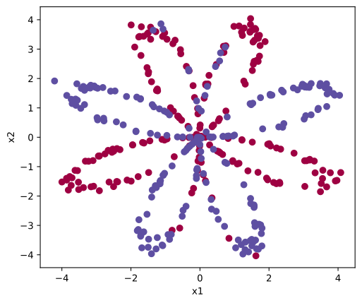

You have

a numpy array (matrix) X that contains your features (x1, x2),
a numpy array (vector) Y that contains your labels (red: 0, blue: 1).

First, get a better sense of what the data is like. How many training examples are there, and what are the shapes of X and Y?

shape_X = X.shape
shape_Y = Y.shape
m = X.shape[1]  # training set size

print('The shape of X is: ' + str(shape_X))
print('The shape of Y is: ' + str(shape_Y))
print('I have m = %d training examples!' % (m))

The shape of X is: (2, 400)
The shape of Y is: (1, 400)
I have m = 400 training examples!

Just as the course notation prescribes, \(X\) is \(n_x \times m\) with one example per column (\(n_x = 2\) here), and \(Y\) is \(1 \times m\).

Simple Logistic Regression

Before building a full neural network, see how logistic regression performs on this problem. sklearn’s built-in LogisticRegressionCV trains a logistic regression classifier in two lines. (sklearn expects examples in rows, hence the transposes.)

# Train the logistic regression classifier
clf = sklearn.linear_model.LogisticRegressionCV()
clf.fit(X.T, Y.T.ravel())

LogisticRegressionCV()

In a Jupyter environment, please rerun this cell to show the HTML representation or trust the notebook.
On GitHub, the HTML representation is unable to render, please try loading this page with nbviewer.org.

LogisticRegressionCV

?Documentation for LogisticRegressionCViFitted

Parameters

	Cs Cs: int or list of floats, default=10 Each of the values in Cs describes the inverse of regularization strength. If Cs is as an int, then a grid of Cs values are chosen in a logarithmic scale between 1e-4 and 1e4. Like in support vector machines, smaller values specify stronger regularization.	10
	l1_ratios l1_ratios: array-like of shape (n_l1_ratios), default=None Floats between 0 and 1 passed as Elastic-Net mixing parameter (scaling between L1 and L2 penalties). For `l1_ratio = 0` the penalty is an L2 penalty. For `l1_ratio = 1` it is an L1 penalty. For `0 < l1_ratio < 1`, the penalty is a combination of L1 and L2. All the values of the given array-like are tested by cross-validation and the one giving the best prediction score is used. .. warning:: Certain values of `l1_ratios`, i.e. some penalties, may not work with some solvers. See the parameter `solver` below, to know the compatibility between the penalty and solver. .. deprecated:: 1.8 `l1_ratios=None` is deprecated in 1.8 and will raise an error in version 1.10. Default value will change from `None` to `(0.0,)` in version 1.10.	'warn'
	fit_intercept fit_intercept: bool, default=True Specifies if a constant (a.k.a. bias or intercept) should be added to the decision function.	True
	cv cv: int or cross-validation generator, default=None The default cross-validation generator used is Stratified K-Folds. If an integer is provided, it specifies the number of folds, `n_folds`, used. See the module :mod:`sklearn.model_selection` module for the list of possible cross-validation objects. .. versionchanged:: 0.22 ``cv`` default value if None changed from 3-fold to 5-fold.	None
	dual dual: bool, default=False Dual (constrained) or primal (regularized, see also :ref:`this equation <regularized-logistic-loss>`) formulation. Dual formulation is only implemented for l2 penalty with liblinear solver. Prefer dual=False when n_samples > n_features.	False
	penalty penalty: {'l1', 'l2', 'elasticnet'}, default='l2' Specify the norm of the penalty: - `'l2'`: add an L2 penalty term (used by default); - `'l1'`: add an L1 penalty term; - `'elasticnet'`: both L1 and L2 penalty terms are added. .. warning:: Some penalties may not work with some solvers. See the parameter `solver` below, to know the compatibility between the penalty and solver. .. deprecated:: 1.8 `penalty` was deprecated in version 1.8 and will be removed in 1.10. Use `l1_ratio` and `C` instead. `l1_ratio=0` for `penalty='l2'`, `l1_ratio=1` for `penalty='l1'`, `l1_ratio` set to any float between 0 and 1 for `penalty='elasticnet'`, and `C=np.inf` for `penalty=None`.	'deprecated'
	scoring scoring: str or callable, default=None The scoring method to use for cross-validation. Options: - str: see :ref:`scoring_string_names` for options. - callable: a scorer callable object (e.g., function) with signature ``scorer(estimator, X, y)``. See :ref:`scoring_callable` for details. - `None`: :ref:`accuracy <accuracy_score>` is used. .. versionchanged:: 1.11 The default will change from None, i.e. accuracy, to 'neg_log_loss' in version 1.11.	'warn'
	solver solver: {'lbfgs', 'liblinear', 'newton-cg', 'newton-cholesky', 'sag', 'saga'}, default='lbfgs' Algorithm to use in the optimization problem. Default is 'lbfgs'. To choose a solver, you might want to consider the following aspects: - 'lbfgs' is a good default solver because it works reasonably well for a wide class of problems. - For :term:`multiclass` problems (`n_classes >= 3`), all solvers except 'liblinear' minimize the full multinomial loss, 'liblinear' will raise an error. - 'newton-cholesky' is a good choice for `n_samples` >> `n_features * n_classes`, especially with one-hot encoded categorical features with rare categories. Be aware that the memory usage of this solver has a quadratic dependency on `n_features * n_classes` because it explicitly computes the full Hessian matrix. - For small datasets, 'liblinear' is a good choice, whereas 'sag' and 'saga' are faster for large ones; - 'liblinear' might be slower in :class:`LogisticRegressionCV` because it does not handle warm-starting. - 'liblinear' can only handle binary classification by default. To apply a one-versus-rest scheme for the multiclass setting one can wrap it with the :class:`~sklearn.multiclass.OneVsRestClassifier`. .. warning:: The choice of the algorithm depends on the penalty (`l1_ratio=0` for L2-penalty, `l1_ratio=1` for L1-penalty and `0 < l1_ratio < 1` for Elastic-Net) chosen and on (multinomial) multiclass support: ================= ======================== ====================== solver l1_ratio multinomial multiclass ================= ======================== ====================== 'lbfgs' l1_ratio=0 yes 'liblinear' l1_ratio=1 or l1_ratio=0 no 'newton-cg' l1_ratio=0 yes 'newton-cholesky' l1_ratio=0 yes 'sag' l1_ratio=0 yes 'saga' 0<=l1_ratio<=1 yes ================= ======================== ====================== .. note:: 'sag' and 'saga' fast convergence is only guaranteed on features with approximately the same scale. You can preprocess the data with a scaler from :mod:`sklearn.preprocessing`. .. versionadded:: 0.17 Stochastic Average Gradient (SAG) descent solver. Multinomial support in version 0.18. .. versionadded:: 0.19 SAGA solver. .. versionadded:: 1.2 newton-cholesky solver. Multinomial support in version 1.6.	'lbfgs'
	tol tol: float, default=1e-4 Tolerance for stopping criteria.	0.0001
	max_iter max_iter: int, default=100 Maximum number of iterations of the optimization algorithm.	100
	class_weight class_weight: dict or 'balanced', default=None Weights associated with classes in the form ``{class_label: weight}``. If not given, all classes are supposed to have weight one. The "balanced" mode uses the values of y to automatically adjust weights inversely proportional to class frequencies in the input data as ``n_samples / (n_classes * np.bincount(y))``. Note that these weights will be multiplied with sample_weight (passed through the fit method) if sample_weight is specified. .. versionadded:: 0.17 class_weight == 'balanced'	None
	n_jobs n_jobs: int, default=None Number of CPU cores used during the cross-validation loop. ``None`` means 1 unless in a :obj:`joblib.parallel_backend` context. ``-1`` means using all processors. See :term:`Glossary <n_jobs>` for more details.	None
	verbose verbose: int, default=0 For the 'liblinear', 'sag' and 'lbfgs' solvers set verbose to any positive number for verbosity.	0
	refit refit: bool, default=True If set to True, the scores are averaged across all folds, and the coefs and the C that corresponds to the best score is taken, and a final refit is done using these parameters. Otherwise the coefs, intercepts and C that correspond to the best scores across folds are averaged.	True
	intercept_scaling intercept_scaling: float, default=1 Useful only when the solver `liblinear` is used and `self.fit_intercept` is set to `True`. In this case, `x` becomes `[x, self.intercept_scaling]`, i.e. a "synthetic" feature with constant value equal to `intercept_scaling` is appended to the instance vector. The intercept becomes ``intercept_scaling * synthetic_feature_weight``. .. note:: The synthetic feature weight is subject to L1 or L2 regularization as all other features. To lessen the effect of regularization on synthetic feature weight (and therefore on the intercept) `intercept_scaling` has to be increased.	1.0
	random_state random_state: int, RandomState instance, default=None Used when `solver='sag'`, 'saga' or 'liblinear' to shuffle the data. Note that this only applies to the solver and not the cross-validation generator. See :term:`Glossary <random_state>` for details.	None
	use_legacy_attributes use_legacy_attributes: bool, default=True If True, use legacy values for attributes: - `C_` is an ndarray of shape (n_classes,) with the same value repeated - `l1_ratio_` is an ndarray of shape (n_classes,) with the same value repeated - `coefs_paths_` is a dict with class labels as keys and ndarrays as values - `scores_` is a dict with class labels as keys and ndarrays as values - `n_iter_` is an ndarray of shape (1, n_folds, n_cs) or similar If False, use new values for attributes: - `C_` is a float - `l1_ratio_` is a float - `coefs_paths_` is an ndarray of shape (n_folds, n_l1_ratios, n_cs, n_classes, n_features) For binary problems (n_classes=2), the 2nd last dimension is 1. - `scores_` is an ndarray of shape (n_folds, n_l1_ratios, n_cs) - `n_iter_` is an ndarray of shape (n_folds, n_l1_ratios, n_cs) .. versionchanged:: 1.10 The default will change from True to False in version 1.10. .. deprecated:: 1.10 `use_legacy_attributes` will be deprecated in version 1.10 and be removed in 1.12.	'warn'

Fitted attributes

Name	Type	Value
C_ C_: ndarray of shape (n_classes,) or (1,) The value of C that maps to the best score, repeated n_classes times. If refit is set to False, the best C is the average of the C's that correspond to the best score for each fold. `C_` is of shape (1,) when the problem is binary. See also parameter `use_legacy_attributes`.	ndarray[float64](1,)	[0.36]
Cs_ Cs_: ndarray of shape (n_cs) Array of C i.e. inverse of regularization parameter values used for cross-validation.	ndarray[float64](10,)	[ 0. , 0. , 0.01,..., 166.81, 1291.55,10000. ]
classes_ classes_: ndarray of shape (n_classes, ) A list of class labels known to the classifier.	ndarray[uint8](2,)	[0,1]
coef_ coef_: ndarray of shape (1, n_features) or (n_classes, n_features) Coefficient of the features in the decision function. `coef_` is of shape (1, n_features) when the given problem is binary.	ndarray[float64](1, 2)	[[ 0.03,-0.2 ]]
coefs_paths_ coefs_paths_: dict of ndarray of shape (n_folds, n_cs, n_dof) or (n_folds, n_cs, n_l1_ratios, n_dof) A dict with classes as the keys, and the path of coefficients obtained during cross-validating across each fold (`n_folds`) and then across each Cs (`n_cs`). The size of the coefficients is the number of degrees of freedom (`n_dof`), i.e. without intercept `n_dof=n_features` and with intercept `n_dof=n_features+1`. If `penalty='elasticnet'`, there is an additional dimension for the number of l1_ratio values (`n_l1_ratios`), which gives a shape of ``(n_folds, n_cs, n_l1_ratios_, n_dof)``. See also parameter `use_legacy_attributes`.	dict	{np.uint8(1): array([[[ 4.2...167067e-04]]])}
intercept_ intercept_: ndarray of shape (1,) or (n_classes,) Intercept (a.k.a. bias) added to the decision function. If `fit_intercept` is set to False, the intercept is set to zero. `intercept_` is of shape (1,) when the problem is binary.	ndarray[float64](1,)	[0.02]
l1_ratio_ l1_ratio_: ndarray of shape (n_classes,) or (n_classes - 1,) The value of l1_ratio that maps to the best score, repeated n_classes times. If refit is set to False, the best l1_ratio is the average of the l1_ratio's that correspond to the best score for each fold. `l1_ratio_` is of shape (1,) when the problem is binary. See also parameter `use_legacy_attributes`.	ndarray[object](1,)	[None]
l1_ratios_ l1_ratios_: ndarray of shape (n_l1_ratios) Array of l1_ratios used for cross-validation. If l1_ratios=None is used (i.e. penalty is not 'elasticnet'), this is set to ``[None]``	ndarray[object](1,)	[None]
n_features_in_ n_features_in_: int Number of features seen during :term:`fit`. .. versionadded:: 0.24	int	2
n_iter_ n_iter_: ndarray of shape (1, n_folds, n_cs) or (1, n_folds, n_cs, n_l1_ratios) Actual number of iterations for all classes, folds and Cs. If `penalty='elasticnet'`, the shape is `(1, n_folds, n_cs, n_l1_ratios)`. See also parameter `use_legacy_attributes`.	ndarray[int32](1, 5, 10)	[[[2,7,6,...,0,0,0], [5,5,6,...,0,0,0], [7,7,6,...,0,0,0], [2,7,5,...,0,0,0], [2,2,3,...,0,0,0]]]
scores_ scores_: dict A dict with classes as the keys, and the values as the grid of scores obtained during cross-validating each fold. The same score is repeated across all classes. Each dict value has shape ``(n_folds, n_cs)`` or ``(n_folds, n_cs, n_l1_ratios)`` if ``penalty='elasticnet'``. See also parameter `use_legacy_attributes`.	dict	{np.uint8(1): array([[0.287...25 , 0.625 ]])}

Now plot the decision boundary of the trained model and print its accuracy.

# Plot the decision boundary for logistic regression
plt.figure(figsize=(6, 5))
plot_decision_boundary(lambda x: clf.predict(x), X, Y)
plt.title("Logistic Regression")

# Print accuracy
LR_predictions = clf.predict(X.T)
accuracy = (np.dot(Y, LR_predictions) + np.dot(1 - Y, 1 - LR_predictions)).item() / Y.size * 100
print('Accuracy of logistic regression: %d ' % accuracy +
      '% ' + "(percentage of correctly labeled datapoints)")

Accuracy of logistic regression: 47 % (percentage of correctly labeled datapoints)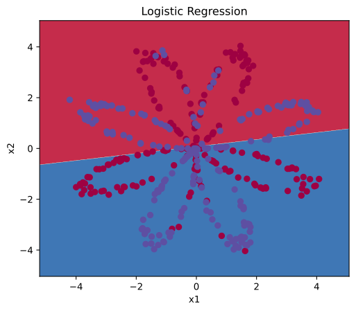

Interpretation. The dataset is not linearly separable, and logistic regression can only draw a straight line, so it does not perform well. Accuracy is 47%, which is below the 50% a constant guess would score on this deliberately balanced dataset (200 examples of each class). Hopefully a neural network will do better.

Neural Network Model

Logistic regression did not work well on the flower dataset. Next, you train a neural network with a single hidden layer and see how it handles the same problem. Here is the model, four tanh units in the hidden layer feeding one sigmoid output unit.

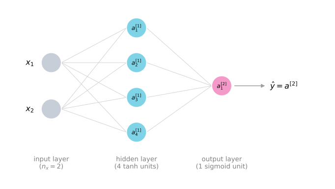
Mathematically, for one example \(x^{(i)}\),

\[ z^{[1](i)} = W^{[1]} x^{(i)} + b^{[1]} \qquad a^{[1](i)} = \tanh\big(z^{[1](i)}\big) \]

\[ z^{[2](i)} = W^{[2]} a^{[1](i)} + b^{[2]} \qquad \hat{y}^{(i)} = a^{[2](i)} = \sigma\big(z^{[2](i)}\big) \]

\[ y^{(i)}_{\text{prediction}} = \begin{cases} 1 & \text{if } a^{[2](i)} > 0.5 \\ 0 & \text{otherwise} \end{cases} \]

Given the predictions on all the examples, you can also compute the cost \(J\) as

\[ J = -\frac{1}{m} \sum_{i=1}^{m} \Big( y^{(i)} \log\big(a^{[2](i)}\big) + \big(1 - y^{(i)}\big) \log\big(1 - a^{[2](i)}\big) \Big) \]

Reminder. The general methodology to build a neural network is

define the neural network structure (number of input units, number of hidden units, and so on),
initialize the model’s parameters,
loop over forward propagation, the loss, backward propagation to get the gradients, and the parameter update (gradient descent).

In practice you build helper functions for each of these steps, then merge them into one function called nn_model(). Once you have built nn_model() and learned the right parameters, you can make predictions on new data.

Defining the Neural Network Structure

Define three variables. n_x is the size of the input layer, n_h is the size of the hidden layer (hard coded to 4 for now), and n_y is the size of the output layer. The input and output sizes come straight from the shapes of X and Y, so this function works for any dataset following the columns-are-examples convention.

def layer_sizes(X, Y):
    """
    Arguments:
    X -- input dataset of shape (input size, number of examples)
    Y -- labels of shape (output size, number of examples)

    Returns:
    n_x -- the size of the input layer
    n_h -- the size of the hidden layer
    n_y -- the size of the output layer
    """
    n_x = X.shape[0]
    n_h = 4
    n_y = Y.shape[0]
    return (n_x, n_h, n_y)

(n_x, n_h, n_y) = layer_sizes(X, Y)
print("The size of the input layer is: n_x = " + str(n_x))
print("The size of the hidden layer is: n_h = " + str(n_h))
print("The size of the output layer is: n_y = " + str(n_y))

The size of the input layer is: n_x = 2
The size of the hidden layer is: n_h = 4
The size of the output layer is: n_y = 1

Initializing the Parameters

Initialize the weight matrices with small random values and the bias vectors with zeros, exactly as the random initialization section explained. If the weights started at zero, every hidden unit would compute the same function forever; random weights break the symmetry, and the 0.01 factor keeps the tanh units away from their flat, saturated regions.

The shapes follow the dimension rules, so \(W^{[1]}\) is \((n_h, n_x)\), \(b^{[1]}\) is \((n_h, 1)\), \(W^{[2]}\) is \((n_y, n_h)\), and \(b^{[2]}\) is \((n_y, 1)\).

def initialize_parameters(n_x, n_h, n_y):
    """
    Argument:
    n_x -- size of the input layer
    n_h -- size of the hidden layer
    n_y -- size of the output layer

    Returns:
    params -- python dictionary containing your parameters:
                    W1 -- weight matrix of shape (n_h, n_x)
                    b1 -- bias vector of shape (n_h, 1)
                    W2 -- weight matrix of shape (n_y, n_h)
                    b2 -- bias vector of shape (n_y, 1)
    """
    W1 = np.random.randn(n_h, n_x) * 0.01
    b1 = np.zeros((n_h, 1))
    W2 = np.random.randn(n_y, n_h) * 0.01
    b2 = np.zeros((n_y, 1))

    parameters = {"W1": W1,
                  "b1": b1,
                  "W2": W2,
                  "b2": b2}

    return parameters

np.random.seed(2)
parameters = initialize_parameters(n_x, n_h, n_y)
print("W1 = " + str(parameters["W1"]))
print("b1 = " + str(parameters["b1"]))
print("W2 = " + str(parameters["W2"]))
print("b2 = " + str(parameters["b2"]))

W1 = [[-0.00416758 -0.00056267]
 [-0.02136196  0.01640271]
 [-0.01793436 -0.00841747]
 [ 0.00502881 -0.01245288]]
b1 = [[0.]
 [0.]
 [0.]
 [0.]]
W2 = [[-0.01057952 -0.00909008  0.00551454  0.02292208]]
b2 = [[0.]]

Forward Propagation

Implement the forward pass using the vectorized equations, tanh for the hidden layer and sigmoid for the output,

\[ Z^{[1]} = W^{[1]} X + b^{[1]} \qquad A^{[1]} = \tanh\big(Z^{[1]}\big) \qquad Z^{[2]} = W^{[2]} A^{[1]} + b^{[2]} \qquad \hat{Y} = A^{[2]} = \sigma\big(Z^{[2]}\big) \]

The function retrieves each parameter from the dictionary, computes the four quantities, and stores \(Z^{[1]}, A^{[1]}, Z^{[2]}, A^{[2]}\) in a cache. Backpropagation will need these values, so the cache is handed to the backward function later rather than recomputing them.

def forward_propagation(X, parameters):
    """
    Argument:
    X -- input data of size (n_x, m)
    parameters -- python dictionary containing your parameters (output of initialization function)

    Returns:
    A2 -- The sigmoid output of the second activation
    cache -- a dictionary containing "Z1", "A1", "Z2" and "A2"
    """
    # Retrieve each parameter from the dictionary "parameters"
    W1 = parameters["W1"]
    b1 = parameters["b1"]
    W2 = parameters["W2"]
    b2 = parameters["b2"]

    # Implement forward propagation to calculate A2 (probabilities)
    Z1 = np.dot(W1, X) + b1
    A1 = np.tanh(Z1)
    Z2 = np.dot(W2, A1) + b2
    A2 = sigmoid(Z2)

    assert(A2.shape == (1, X.shape[1]))

    cache = {"Z1": Z1,
             "A1": A1,
             "Z2": Z2,
             "A2": A2}

    return A2, cache

A2, cache = forward_propagation(X, parameters)
print("A2 shape: " + str(A2.shape))
print("First five predictions: " + str(A2[0, :5]))

A2 shape: (1, 400)
First five predictions: [0.4996522  0.50018609 0.50015804 0.50026729 0.49970121]

With the tiny random initial weights, every prediction sits very close to 0.5, the network has not learned anything yet.

Computing the Cost

Now that you have \(A^{[2]}\) (in the Python variable A2), which contains \(a^{[2](i)}\) for every example, compute the cost. One way to implement part of the sum \(-\sum_{i=1}^{m} y^{(i)} \log\big(a^{[2](i)}\big)\) without a for loop is np.multiply(np.log(A2), Y) followed by np.sum, multiplying the two arrays element by element and adding everything up. The same trick handles the \((1 - y)\) term, and dividing by \(m\) gives the average.

The final float(np.squeeze(cost)) makes sure the cost comes out as a plain number rather than a one by one array (it turns [[17]] into 17).

def compute_cost(A2, Y):
    """
    Computes the cross-entropy cost

    Arguments:
    A2 -- The sigmoid output of the second activation, of shape (1, number of examples)
    Y -- "true" labels vector of shape (1, number of examples)

    Returns:
    cost -- cross-entropy cost
    """
    m = Y.shape[1]  # number of examples

    # Compute the cross-entropy cost
    logprobs = np.multiply(np.log(A2), Y) + np.multiply(np.log(1 - A2), (1 - Y))
    cost = -np.sum(logprobs) / m

    cost = float(np.squeeze(cost))

    return cost

cost = compute_cost(A2, Y)
print("cost = " + str(cost))

cost = 0.6930480201239823

A sanity check worth noticing: with all predictions near 0.5, the cost is close to \(-\log(0.5) \approx 0.693\), exactly what the cross entropy of a coin-flip guess should be.

Backward Propagation

Using the cache computed during forward propagation, you can now implement backward propagation. Backpropagation is usually the hardest, most mathematical part of deep learning. The six vectorized equations are exactly the ones derived on the gradient descent page,

\[ dZ^{[2]} = A^{[2]} - Y \qquad dW^{[2]} = \frac{1}{m} dZ^{[2]} A^{[1]T} \qquad db^{[2]} = \frac{1}{m}\, \texttt{np.sum}\big(dZ^{[2]}, \text{axis=1, keepdims=True}\big) \]

\[ dZ^{[1]} = W^{[2]T} dZ^{[2]} * g^{[1]\prime}\big(Z^{[1]}\big) \qquad dW^{[1]} = \frac{1}{m} dZ^{[1]} X^{T} \qquad db^{[1]} = \frac{1}{m}\, \texttt{np.sum}\big(dZ^{[1]}, \text{axis=1, keepdims=True}\big) \]

One tip: to compute \(dZ^{[1]}\) you need \(g^{[1]\prime}(Z^{[1]})\). Since \(g^{[1]}\) is the tanh activation, its derivative is \(1 - a^2\), so you can compute \(g^{[1]\prime}(Z^{[1]})\) as (1 - np.power(A1, 2)) using the cached A1.

def backward_propagation(parameters, cache, X, Y):
    """
    Implement the backward propagation using the six equations above.

    Arguments:
    parameters -- python dictionary containing our parameters
    cache -- a dictionary containing "Z1", "A1", "Z2" and "A2"
    X -- input data of shape (2, number of examples)
    Y -- "true" labels vector of shape (1, number of examples)

    Returns:
    grads -- python dictionary containing your gradients with respect to different parameters
    """
    m = X.shape[1]

    # Retrieve W1 and W2 from the dictionary "parameters"
    W1 = parameters["W1"]
    W2 = parameters["W2"]

    # Retrieve A1 and A2 from dictionary "cache"
    A1 = cache["A1"]
    A2 = cache["A2"]

    # Backward propagation: calculate dW1, db1, dW2, db2
    dZ2 = A2 - Y
    dW2 = (1 / m) * np.dot(dZ2, A1.T)
    db2 = (1 / m) * np.sum(dZ2, axis=1, keepdims=True)
    dZ1 = np.dot(W2.T, dZ2) * (1 - np.power(A1, 2))
    dW1 = (1 / m) * np.dot(dZ1, X.T)
    db1 = (1 / m) * np.sum(dZ1, axis=1, keepdims=True)

    grads = {"dW1": dW1,
             "db1": db1,
             "dW2": dW2,
             "db2": db2}

    return grads

grads = backward_propagation(parameters, cache, X, Y)
print("dW1 shape: " + str(grads["dW1"].shape))
print("db1 shape: " + str(grads["db1"].shape))
print("dW2 shape: " + str(grads["dW2"].shape))
print("db2 shape: " + str(grads["db2"].shape))

dW1 shape: (4, 2)
db1 shape: (4, 1)
dW2 shape: (1, 4)
db2 shape: (1, 1)

As the dimension-checking rule promises, each dfoo has exactly the same shape as its foo.

Updating the Parameters

Implement the gradient descent update rule. For any parameter \(\theta\),

\[ \theta := \theta - \alpha \frac{\partial J}{\partial \theta} \]

where \(\alpha\) is the learning rate. With a good learning rate the iterates walk steadily downhill to the minimum; with a bad, too-large one they overshoot and can diverge, as illustrated back in the machine learning course’s learning rate discussion.

One Python detail. copy.deepcopy is used when retrieving the weight matrices, so the update builds new arrays instead of silently modifying the dictionaries the caller passed in.

def update_parameters(parameters, grads, learning_rate=1.2):
    """
    Updates parameters using the gradient descent update rule given above

    Arguments:
    parameters -- python dictionary containing your parameters
    grads -- python dictionary containing your gradients

    Returns:
    parameters -- python dictionary containing your updated parameters
    """
    # Retrieve a copy of each parameter from the dictionary "parameters"
    W1 = copy.deepcopy(parameters["W1"])
    b1 = parameters["b1"]
    W2 = copy.deepcopy(parameters["W2"])
    b2 = parameters["b2"]

    # Retrieve each gradient from the dictionary "grads"
    dW1 = grads["dW1"]
    db1 = grads["db1"]
    dW2 = grads["dW2"]
    db2 = grads["db2"]

    # Update rule for each parameter
    W1 = W1 - learning_rate * dW1
    b1 = b1 - learning_rate * db1
    W2 = W2 - learning_rate * dW2
    b2 = b2 - learning_rate * db2

    parameters = {"W1": W1,
                  "b1": b1,
                  "W2": W2,
                  "b2": b2}

    return parameters

Integration: Build nn_model()

Integrate the previous functions into nn_model(), in the right order. Define the sizes, initialize the parameters, then loop over forward propagation, cost, backward propagation, and the parameter update.

def nn_model(X, Y, n_h, num_iterations=10000, print_cost=False):
    """
    Arguments:
    X -- dataset of shape (2, number of examples)
    Y -- labels of shape (1, number of examples)
    n_h -- size of the hidden layer
    num_iterations -- Number of iterations in gradient descent loop
    print_cost -- if True, print the cost every 1000 iterations

    Returns:
    parameters -- parameters learned by the model. They can then be used to predict.
    """
    np.random.seed(3)
    n_x = layer_sizes(X, Y)[0]
    n_y = layer_sizes(X, Y)[2]

    # Initialize parameters
    parameters = initialize_parameters(n_x, n_h, n_y)

    # Loop (gradient descent)
    for i in range(0, num_iterations):

        # Forward propagation. Inputs: "X, parameters". Outputs: "A2, cache".
        A2, cache = forward_propagation(X, parameters)

        # Cost function. Inputs: "A2, Y". Outputs: "cost".
        cost = compute_cost(A2, Y)

        # Backpropagation. Inputs: "parameters, cache, X, Y". Outputs: "grads".
        grads = backward_propagation(parameters, cache, X, Y)

        # Gradient descent parameter update. Inputs: "parameters, grads". Outputs: "parameters".
        parameters = update_parameters(parameters, grads, learning_rate=1.2)

        # Print the cost every 1000 iterations
        if print_cost and i % 1000 == 0:
            print("Cost after iteration %i: %f" % (i, cost))

    return parameters

Test the Model

Predict

Predict with your model by building predict(). It uses forward propagation to compute the probabilities \(A^{[2]}\), then thresholds them at 0.5,

\[ y_{\text{prediction}} = \begin{cases} 1 & \text{if } a^{[2]} > 0.5 \\ 0 & \text{otherwise} \end{cases} \]

In NumPy, comparing a whole array against a threshold does this in one step: (A2 > 0.5) produces an array of True/False values, which behave as 1 and 0.

def predict(parameters, X):
    """
    Using the learned parameters, predicts a class for each example in X

    Arguments:
    parameters -- python dictionary containing your parameters
    X -- input data of size (n_x, m)

    Returns
    predictions -- vector of predictions of our model (red: 0 / blue: 1)
    """
    # Compute probabilities using forward propagation, and classify to 0/1 using 0.5 as the threshold
    A2, cache = forward_propagation(X, parameters)
    predictions = (A2 > 0.5)

    return predictions

Test the Model on the Planar Dataset

It is time to run the model and see how it performs on the planar dataset. Train it with a hidden layer of 4 units for 10,000 iterations of gradient descent, then plot the learned decision boundary.

# Build a model with a n_h-dimensional hidden layer
parameters = nn_model(X, Y, n_h=4, num_iterations=10000, print_cost=True)

# Plot the decision boundary
plt.figure(figsize=(6, 5))
plot_decision_boundary(lambda x: predict(parameters, x.T), X, Y)
plt.title("Decision Boundary for hidden layer size " + str(4))
plt.show()

Cost after iteration 0: 0.693162
Cost after iteration 1000: 0.258625
Cost after iteration 2000: 0.239334
Cost after iteration 3000: 0.230802
Cost after iteration 4000: 0.225528
Cost after iteration 5000: 0.221845
Cost after iteration 6000: 0.219094
Cost after iteration 7000: 0.220617
Cost after iteration 8000: 0.219412
Cost after iteration 9000: 0.218526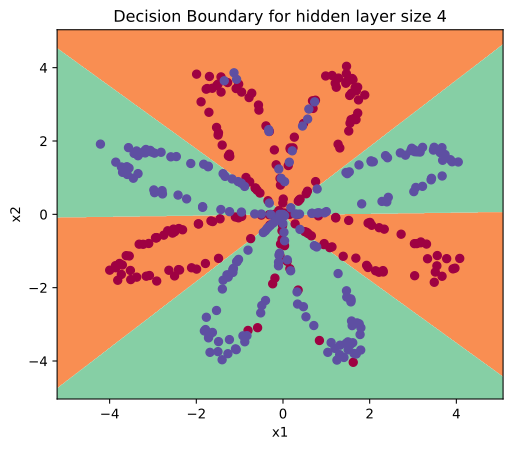

# Print accuracy
predictions = predict(parameters, X)
accuracy = (np.dot(Y, predictions.T) + np.dot(1 - Y, 1 - predictions.T)).item() / Y.size * 100
print('Accuracy: %d' % accuracy + '%')

Accuracy: 90%

Accuracy is really high compared to logistic regression, 90% against 47%. The model has learned the patterns of the flower’s petals. Unlike logistic regression, neural networks are able to learn even highly non-linear decision boundaries, and that difference is exactly what the tanh hidden layer buys you.

What to Remember

A neural network with one hidden layer is built from the same ingredients as logistic regression, a linear step and an activation per layer, applied twice.
The workflow is always the same. Define the structure, initialize the parameters randomly, then loop forward propagation, cost, backward propagation, and the gradient descent update.
The cache saves the forward pass values (\(Z^{[1]}, A^{[1]}, Z^{[2]}, A^{[2]}\)) so backpropagation can reuse them.
tanh hidden units plus a sigmoid output let the network carve non-linear decision boundaries that a linear model can never draw.

Review Questions

1. Why does logistic regression reach only 47% accuracy on the flower dataset while the one hidden layer network reaches 90%?

Answer

Logistic regression can only draw a linear decision boundary, and the flower’s petals are not linearly separable, so no straight line does well. The hidden layer of tanh units lets the network compose non-linear functions of the inputs, carving a petal-shaped boundary that follows the data.

1. In backward_propagation, why can \(g^{[1]\prime}(Z^{[1]})\) be computed as (1 - np.power(A1, 2))?

Answer

The hidden activation is \(\tanh\), whose derivative is \(1 - \tanh(z)^2\). Since the cached A1 already holds \(\tanh(Z^{[1]})\), the derivative comes almost for free as \(1 - (A^{[1]})^2\), applied element-wise, with no need to recompute the tanh.

1. What is the purpose of the cache returned by forward_propagation?

Answer

It stores \(Z^{[1]}, A^{[1]}, Z^{[2]}, A^{[2]}\) from the forward pass. Backpropagation needs exactly these values (for example \(A^{[1]}\) in \(dW^{[2]}\) and \(dZ^{[1]}\)), so caching them avoids recomputing the forward pass during the backward step.

1. Why are the weights initialized with np.random.randn(...) * 0.01 instead of zeros, and why are zero biases fine?

Answer

Zero weights would make every hidden unit compute the same function, and by symmetry their gradients would stay identical forever, so the network could never use more than one effective hidden unit. Small random weights break the symmetry, and the 0.01 factor keeps the tanh units off their flat, saturated regions. The biases do not cause the symmetry problem, so zeros are fine for them.

1. Why does the cost on the freshly initialized network come out near 0.693?

Answer

With tiny random weights, \(Z^{[2]}\) is close to zero and the sigmoid outputs are all close to 0.5, a coin-flip guess for every example. The cross entropy of predicting 0.5 is \(-\log(0.5) = \log 2 \approx 0.693\), so a starting cost near that value is a sign the implementation is correct.