import numpy as np

# Tumor size (cm) vs malignant/benign label
x_train = np.array([0.0, 1, 2, 3, 4, 5])
y_train = np.array([0, 0, 0, 1, 1, 1])Logistic Regression
machine-learning
supervised-learning
classification
For a long time, much of internet advertising was driven by a close cousin of logistic regression. Large websites used models like this to decide which…
For a long time, much of internet advertising was driven by a close cousin of logistic regression. Large websites used models like this to decide which ad to show you. The business details differ, but the core idea is the same in every case. The model estimates the probability of a click or conversion, then the platform acts on that score.
On the classification page you saw why a straight line is a poor fit for yes/no labels. Logistic regression is probably the single most widely used classification algorithm in the world. It outputs a value between 0 and 1 that you can read as the chance of the positive class, then map to a final label of 0 or 1.
We continue with the tumor example: malignant tumors are the positive class (\(y = 1\)), and benign tumors are the negative class (\(y = 0\)).
Review Questions
1. What type of problem is logistic regression designed for?
TipAnswer
Binary classification, where the target \(y\) takes on only two values (such as 0 and 1).
S-Shaped Fit for Classification
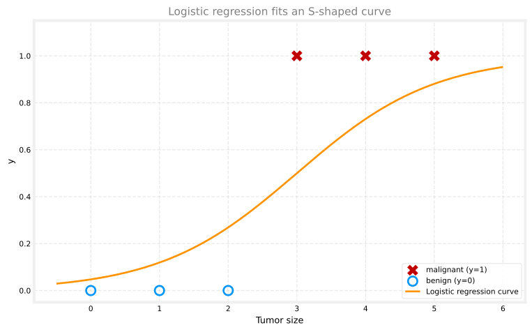
Recall the tumor data: tumor size on the horizontal axis and label \(y\) on the vertical axis (only 0 or 1).
Linear regression is not a good algorithm for this problem. Logistic regression instead fits an S-shaped curve that stays between 0 and 1.
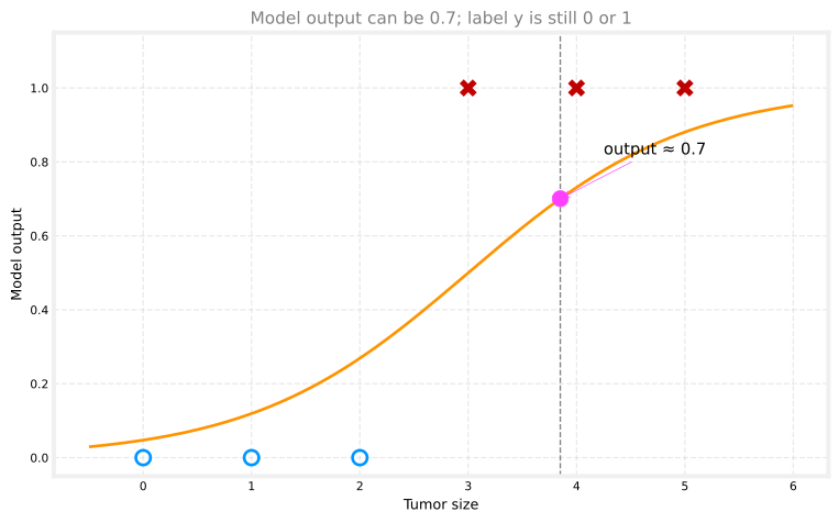
For a patient whose tumor size is marked on the plot below, the model might output 0.7. That number is not the final label. The true label \(y\) is still only ever 0 or 1. The value 0.7 is the model output before you turn it into a class prediction (you will see how later on this page).
Review Questions
1. Can the final training label \(y\) be 0.7 in binary classification?
TipAnswer
No. Labels are 0 or 1. A value like 0.7 is a model output (a probability-like score), not the ground-truth label.
Sigmoid Function
To build logistic regression, you need a function that squashes any real number into the range \((0, 1)\). That function is the sigmoid function, also called the logistic function. We write it as \(g(z)\):
\[ g(z) = \frac{1}{1 + e^{-z}} \]
Here \(e \approx 2.72\) is Euler number, a mathematical constant (like \(\pi\)).
The plot below shows \(g(z)\) for \(z\) between \(-3\) and \(3\). The horizontal axis is labeled \(z\) because this graph is about the input to \(g\), not tumor size directly.
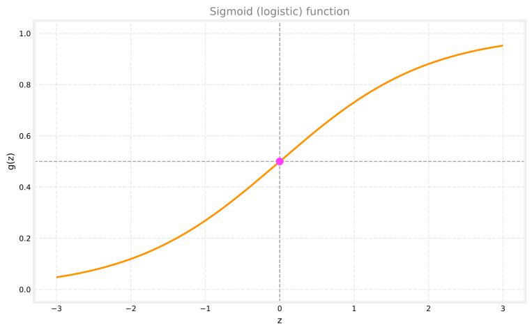
Large positive \(z\): if \(z = 100\), then \(e^{-z}\) is tiny, so \(g(z) \approx \frac{1}{1 + 0} = 1\).
Large negative \(z\): if \(z = -100\), then \(e^{-z}\) is huge, so \(g(z) \approx \frac{1}{\text{giant number}} \approx 0\).
At \(z = 0\): \(e^{-0} = 1\), so \(g(0) = \frac{1}{1 + 1} = 0.5\). That is why the curve crosses the vertical axis at 0.5.
Review Questions
1. What is \(g(0)\) for the sigmoid function?
TipAnswer
0.5, because \(g(0) = \frac{1}{1 + e^{0}} = \frac{1}{2}\).
1. For very large positive \(z\), is \(g(z)\) closer to 0 or to 1?
TipAnswer
Closer to 1. The denominator \(1 + e^{-z}\) approaches 1 when \(e^{-z}\) is tiny.
Logistic Regression Model
Logistic regression is built in two steps.
Step 1: compute a linear score (the same idea as linear regression):
\[ z = \vec{w} \cdot \vec{x} + b \]
For the tumor example with a single feature, \(\vec{x} = [x]\) and this reduces to \(z = wx + b\).
Step 2: pass \(z\) through the sigmoid:
\[ f_{\vec{w},b}(\vec{x}) = g(z) = g(\vec{w} \cdot \vec{x} + b) = \frac{1}{1 + e^{-(\vec{w} \cdot \vec{x} + b)}} \]
The model inputs a feature vector \(\vec{x}\) and outputs a number strictly between 0 and 1 (in practice, very close to 0 or 1 at the extremes, but never exactly 0 or 1 from the formula alone).
for x_val in [0.0, 2.0, 5.0]:
    z_val = w_demo * x_val + b_demo
    print(f"x = {x_val:.1f}  ->  z = {z_val:.1f}  ->  f(x) = {sigmoid(z_val):.3f}")
x = 0.0 -> z = -3.0 -> f(x) = 0.047
x = 2.0 -> z = -1.0 -> f(x) = 0.269
x = 5.0 -> z = 2.0 -> f(x) = 0.881Review Questions
1. In \(f_{\vec{w},b}(\vec{x}) = g(\vec{w} \cdot \vec{x} + b)\), what role does \(g\) play?
TipAnswer
\(g\) is the sigmoid. It maps the linear score \(z = \vec{w} \cdot \vec{x} + b\) into the range \((0, 1)\) so the output can be read as a probability-like value.
Interpreting the Output
Return to tumor classification. A useful way to read logistic regression output is:
\[ f_{w,b}(x) \approx P(y = 1 \mid x) \]
In words: given tumor size \(x\), the model output is the estimated probability that \(y = 1\) (malignant).
Example: if \(f_{w,b}(x) = 0.7\) for a patient, the model estimates a 70% chance that the true label is malignant (\(y = 1\)).
Because \(y\) must be either 0 or 1, the two probabilities add to 100%:
\[ P(y = 1 \mid x) + P(y = 0 \mid x) = 1 \]
So if the chance of \(y = 1\) is 0.7 (70%), the chance of \(y = 0\) is 0.3 (30%).
Review Questions
1. If \(f_{w,b}(x) = 0.7\), how should you interpret that number?
TipAnswer
The model estimates a 70% probability that \(y = 1\) (malignant) for that input \(x\).
1. If \(P(y = 1 \mid x) = 0.7\), what is \(P(y = 0 \mid x)\)?
TipAnswer
0.3 (30%), because the two probabilities must sum to 1.
Notation You May See Elsewhere
In research papers or blog posts, you might see:
\[ f_{w,b}(x) = P(y = 1 \mid x;\, w, b) \]
The semicolon reminds you that \(w\) and \(b\) are parameters that shape the computation. For this course, you do not need to memorize every symbol in that notation. The important idea is simpler. Output \(\approx\) probability of class 1.
Decision Boundary
So far, logistic regression has given you a score between 0 and 1, like 0.7 or 0.3. That number is helpful, but in real use you usually need a clear answer. Should we treat this tumor as malignant or benign? Should we mark this email as spam or not spam?
That final answer is written \(\hat{y}\) (said “y-hat”). It is your prediction, not the true label \(y\) stored in the training data.
The decision boundary is where the model is on the fence between predicting 0 and predicting 1. On one side of the boundary the model leans toward class 0. On the other side it leans toward class 1. With one input feature (such as tumor size), the boundary is a single cutoff on the \(x\) axis. With two features it becomes a line in the \((x_1, x_2)\) plane, and with polynomial features it can even curve.
The sections below walk through the usual cutoff rule, then show what these boundaries look like in pictures.
Threshold at 0.5
Return to the tumor example. The model might output 0.7 for one patient and 0.3 for another. Those values are still probabilities, not final yes/no answers.
To turn a probability into a prediction, compare the model output to a cutoff called a threshold. The standard choice is 0.5, right in the middle of the 0-to-1 range. You can think of it like a pass/fail line at 50% on a test. At or above the line you call it a “pass” (predict class 1). Below the line you call it a “fail” (predict class 0).
- If \(f_{\vec{w},b}(\vec{x}) \ge 0.5\), the model is at least half convinced that \(y = 1\), so predict \(\hat{y} = 1\).
- If \(f_{\vec{w},b}(\vec{x}) < 0.5\), the model leans toward \(y = 0\), so predict \(\hat{y} = 0\).
Example: with a 0.5 threshold, an output of 0.7 gives \(\hat{y} = 1\) (malignant). An output of 0.3 gives \(\hat{y} = 0\) (benign).
\(\hat{y}\) is what the model guesses for a new example. The true label \(y\) from the dataset can still be 0 or 1, and the model can be right or wrong.
Review Questions
1. If \(f_{\vec{w},b}(\vec{x}) = 0.65\), what is \(\hat{y}\) with a 0.5 threshold?
TipAnswer
\(\hat{y} = 1\), because \(0.65 \ge 0.5\).
When Does the Model Predict 1?
When is \(f_{\vec{w},b}(\vec{x}) \ge 0.5\)? Work through the chain:
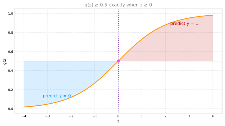
- \(f_{\vec{w},b}(\vec{x}) = g(z)\), so you need \(g(z) \ge 0.5\).
- The sigmoid equals 0.5 at \(z = 0\) and rises toward 1 for larger \(z\). So \(g(z) \ge 0.5\) when \(z \ge 0\).
- \(z = \vec{w} \cdot \vec{x} + b\), so you need \(\vec{w} \cdot \vec{x} + b \ge 0\).
Putting those steps together, the prediction rule can be written directly in terms of \(z\).
\[ \hat{y} = 1 \quad \text{when} \quad \vec{w} \cdot \vec{x} + b \ge 0 \]
\[ \hat{y} = 0 \quad \text{when} \quad \vec{w} \cdot \vec{x} + b < 0 \]
Review Questions
1. With a 0.5 threshold, when does logistic regression predict \(\hat{y} = 1\)?
TipAnswer
When \(z = \vec{w} \cdot \vec{x} + b \ge 0\) (equivalently, when \(f_{\vec{w},b}(\vec{x}) \ge 0.5\)).
Linear Decision Boundary (Two Features)
Consider two features \(x_1\) and \(x_2\). First compute the linear score \(z\) as a weighted sum of those features.
\[ z = w_1 x_1 + w_2 x_2 + b \]
You can write the same expression with vectors. Collect the features into \(\vec{x} = \begin{bmatrix} x_1 \\ x_2 \end{bmatrix}\) and the weights into \(\vec{w} = \begin{bmatrix} w_1 \\ w_2 \end{bmatrix}\). Then the dot product expands to the same sum.
\[ z = \vec{w} \cdot \vec{x} + b \]
Now plug in numbers. Let \(w_1 = 1\), \(w_2 = 1\), and \(b = -3\). The model predicts \(\hat{y} = 1\) whenever the score is non-negative, which in this case means
\[ x_1 + x_2 - 3 \ge 0 \]
The decision boundary is the border where the model is exactly neutral between the two classes. On that border the score is zero, because \(z = 0\) is where the sigmoid output hits the 0.5 threshold. In general, the decision boundary is defined by
\[ \vec{w} \cdot \vec{x} + b = 0 \]
For \(w_1 = 1\), \(w_2 = 1\), and \(b = -3\), this becomes
\[ x_1 + x_2 - 3 = 0 \]
which rearranges to the line
\[ x_1 + x_2 = 3 \]
On one side of this line the model predicts \(\hat{y} = 1\). On the other side it predicts \(\hat{y} = 0\).
X_db = np.array([[0.5, 1.5], [1.0, 1.0], [1.5, 0.5], [3.0, 0.5], [2.0, 2.0], [1.0, 2.5]])
y_db = np.array([0, 0, 0, 1, 1, 1])
w1, w2, b_db = 1.0, 1.0, -3.0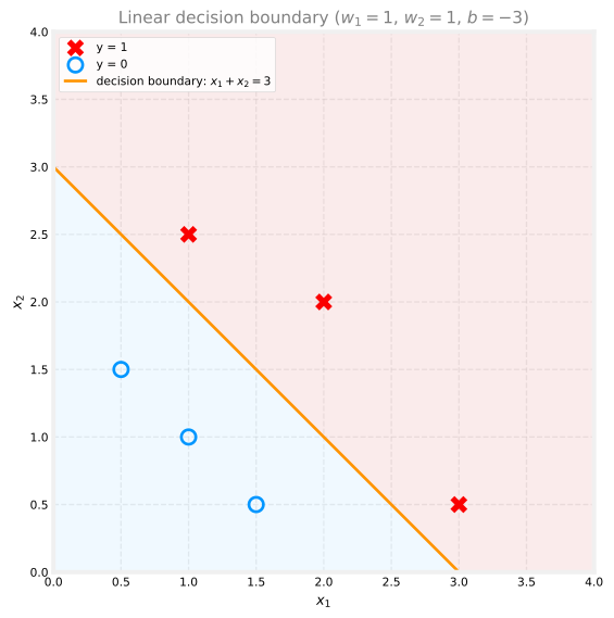
Points to the right and above the line (where \(x_1 + x_2 \ge 3\)) get \(\hat{y} = 1\). Points to the left and below get \(\hat{y} = 0\). Different parameters \(\vec{w}\) and \(b\) would give a different boundary line.
Review Questions
1. For \(w_1 = 1\), \(w_2 = 1\), \(b = -3\), what equation defines the decision boundary?
TipAnswer
\(x_1 + x_2 = 3\), from setting \(\vec{w} \cdot \vec{x} + b = 0\).
Non-Linear Decision Boundaries
If you use only \(x_1\) and \(x_2\) as features, the decision boundary is always a straight line (in two dimensions). To bend the boundary, engineer polynomial features, just as in feature engineering and polynomial regression.
Use squared terms in the score. Instead of weighting \(x_1\) and \(x_2\) directly, weight their squares.
\[ z = w_1 x_1^2 + w_2 x_2^2 + b \]
Then pass \(z\) through the sigmoid as usual, so \(f_{\vec{w},b}(\vec{x}) = g(z)\).
With \(w_1 = 1\), \(w_2 = 1\), and \(b = -1\), the score simplifies to
\[ z = x_1^2 + x_2^2 - 1 \]
The decision boundary is still where the score equals zero. Set \(z = 0\) and solve.
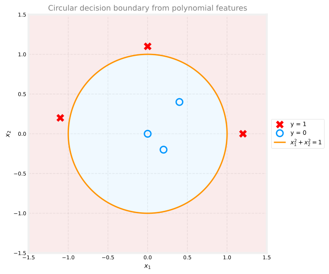
\[ x_1^2 + x_2^2 = 1 \]
That is a circle of radius 1. The model predicts \(\hat{y} = 1\) outside the circle (where \(x_1^2 + x_2^2 \ge 1\)) and \(\hat{y} = 0\) inside.
Even More Complex Boundaries
You can add higher-order terms, such as \(x_1^2\), \(x_1 x_2\), and \(x_2^2\) together:
\[ z = w_1 x_1 + w_2 x_2 + w_3 x_1^2 + w_4 x_1 x_2 + w_5 x_2^2 + b \]
With the right weights, the decision boundary (where \(z = 0\)) can become an ellipse or an even more intricate curve. Logistic regression can therefore fit fairly complex regions: predict \(\hat{y} = 1\) inside one shape and \(\hat{y} = 0\) outside.
The trade-off is that more polynomial features give more flexible boundaries, but also more parameters to learn and more risk of overfitting (covered later in the course).
Key takeaway: if you use only the original features \(x_1, x_2, \ldots\) with no engineered powers or cross-terms, the decision boundary stays linear. Polynomial (and other engineered) features are what let the boundary bend.
Review Questions
1. True or false? With only features \(x_1\) and \(x_2\) (no engineered terms), the logistic regression decision boundary in the \((x_1, x_2)\) plane is always a straight line.
TipAnswer
True. The boundary is \(\vec{w} \cdot \vec{x} + b = 0\), which is linear in \(x_1\) and \(x_2\).
1. Why does \(z = x_1^2 + x_2^2 - 1\) produce a circular decision boundary?
TipAnswer
Setting \(z = 0\) gives \(x_1^2 + x_2^2 = 1\), the equation of a circle. The model flips between \(\hat{y} = 0\) and \(\hat{y} = 1\) on that curve.
Lab: Decision Boundary
In this lab you will plot a logistic regression decision boundary for a two-feature data set. You will see exactly where the model switches from predicting \(\hat{y} = 0\) to \(\hat{y} = 1\).
Goals
In this lab, you will:
- plot a two-feature classification data set
- visualize the sigmoid threshold at \(z = 0\)
- draw the decision boundary for a trained model and shade the two prediction regions
Tools
You will use NumPy, Matplotlib, and the same \(x_1\) / \(x_2\) feature names as earlier on this page.
Dataset
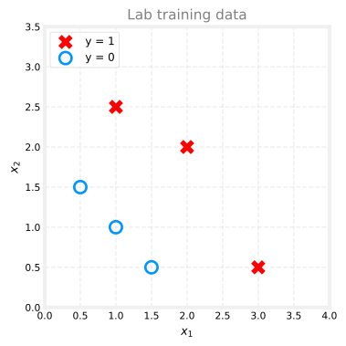
The training set has six examples. Each row of X has two features. The target y is 0 or 1.
import numpy as np
import matplotlib.pyplot as plt
from matplotlib.patches import FancyArrowPatch

plt.style.use("../../deeplearning.mplstyle")

dlblue = "#0096ff"
dldarkred = "#C00000"

X_lab = np.array([[0.5, 1.5], [1.0, 1.0], [1.5, 0.5], [3.0, 0.5], [2.0, 2.0], [1.0, 2.5]])
y_lab = np.array([0, 0, 0, 1, 1, 1])


def plot_data(X, y, ax):
    pos = y.reshape(-1) == 1
    neg = y.reshape(-1) == 0
    ax.scatter(X[pos, 0], X[pos, 1], marker="x", s=80, c="red", label="y = 1")
    ax.scatter(X[neg, 0], X[neg, 1], marker="o", s=100, facecolors="none",
               edgecolors=dlblue, linewidths=2, label="y = 0")
    ax.legend(loc="upper left", fontsize=9)
Red X marks are \(y = 1\). Blue circles are \(y = 0\).
Trained Model (Given Parameters)
Suppose you already trained logistic regression on this data and obtained
\[ f_{\vec{w},b}(\vec{x}) = g(w_1 x_1 + w_2 x_2 + b) \]
with \(w_1 = 1\), \(w_2 = 1\), and \(b = -3\). You will learn how to fit these values from data later in the course. For now, use them to study the decision boundary.
In this example the score is
\[ z = x_1 + x_2 - 3 \]
so \(f_{\vec{w},b}(\vec{x}) = g(x_1 + x_2 - 3)\).
Sigmoid Threshold at \(z = 0\)
The model predicts \(\hat{y} = 1\) when \(f_{\vec{w},b}(\vec{x}) \ge 0.5\), which happens when \(z \ge 0\). The plot below shows the sigmoid and marks the split at \(z = 0\).
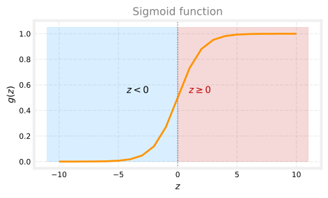
Because \(z = \vec{w} \cdot \vec{x} + b\) for logistic regression, the model predicts \(\hat{y} = 1\) when \(\vec{w} \cdot \vec{x} + b \ge 0\) and \(\hat{y} = 0\) when that score is negative.
Plotting the Decision Boundary
For \(w_1 = 1\), \(w_2 = 1\), and \(b = -3\), the model predicts \(\hat{y} = 1\) when
\[ x_1 + x_2 - 3 \ge 0 \]
The decision boundary is where the score equals zero. Set \(x_1 + x_2 - 3 = 0\) and solve for \(x_2\) to get a line you can plot.
\[ x_2 = 3 - x_1 \]
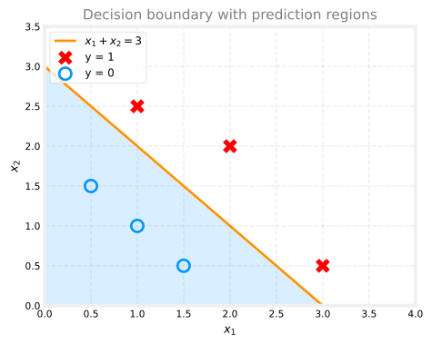
The orange line is \(x_1 + x_2 - 3 = 0\). It crosses the \(x_2\) axis at \((0, 3)\) and the \(x_1\) axis at \((3, 0)\).
The shaded region below the line is where \(x_1 + x_2 - 3 < 0\), so the model predicts \(\hat{y} = 0\). The region on or above the line is where the score is non-negative, so the model predicts \(\hat{y} = 1\). That line is the decision boundary.
As you saw earlier on this page, higher-order polynomial features can bend this boundary into curves such as circles or ellipses.
Lab Summary
In this lab you:
- plotted a two-feature classification data set
- connected the 0.5 sigmoid threshold to the condition \(z \ge 0\)
- drew the decision boundary \(x_1 + x_2 = 3\) and identified which side predicts each class
Review Questions
1. Which is an example of a classification task?
Based on the size of each tumor, determine if each tumor is malignant (cancerous) or not.
Based on a patient’s blood pressure, determine how much blood pressure medication (a dosage measured in milligrams) the patient should be prescribed.
Based on a patient’s age and blood pressure, determine how much blood pressure medication (measured in milligrams) the patient should be prescribed.
TipAnswer
a. The output is a category (malignant or not). Options b and c predict a number (milligrams of medication), which is regression.
1. Recall the sigmoid function is \(g(z) = \frac{1}{1 + e^{-z}}\). If \(z\) is a large positive number, then:
\(g(z)\) is near \(-1\)
\(g(z)\) is near \(1\)
\(g(z)\) will be near \(0.5\)
\(g(z)\) will be near \(0\)
TipAnswer
b. When \(z\) is large and positive, \(e^{-z}\) is tiny, so \(g(z) \approx \frac{1}{1 + 0} = 1\).
1. A cat photo classification model predicts 1 if it is a cat, and 0 if it is not a cat. For a particular photograph, the logistic regression model outputs \(g(z)\) (a number between 0 and 1). Which of these would be a reasonable criterion to decide whether to predict that it is a cat?
Predict it is a cat if \(g(z) = 0.5\)
Predict it is a cat if \(g(z) < 0.5\)
Predict it is a cat if \(g(z) \ge 0.5\)
Predict it is a cat if \(g(z) < 0.7\)
TipAnswer
c. The usual threshold is 0.5. Predict class 1 when the model output is at or above that cutoff, so predict “cat” when \(g(z) \ge 0.5\).
1. True or false? No matter what features you use (including polynomial features), the decision boundary learned by logistic regression will be a linear decision boundary.
True
False
TipAnswer
b. False. With only the original features \(x_1, x_2, \ldots\), the boundary is linear. Polynomial features (such as \(x_1^2\) and \(x_2^2\)) let the boundary bend into curves like circles or ellipses in the \((x_1, x_2)\) plane.
What Comes Next
You now know the logistic regression model, how to read its output as a probability, and how the decision boundary turns scores like 0.3 or 0.7 into predictions \(\hat{y} = 0\) or \(\hat{y} = 1\).
The next step is training. The next page introduces the cost function for logistic regression, then you will see a compact form of that cost and gradient descent to minimize it.