A real neural network trained on 1000 real handwritten digit images to tell zeros from ones, built with the same Sequential pattern from the previous pages.
Published
July 11, 2026
Earlier pages used a small schematic 8-by-8 digit example to introduce the forward propagation architecture, 64 pixels feeding a 25-15-1 network. This lab uses that same idea for real, on 1000 real handwritten digit images, each 20 by 20 pixels, to build a neural network that tells the digits zero and one apart. It reuses the exact same Sequential, Dense, compile, fit, and predict pattern already taught on the TensorFlow Implementation page, applied here to real image data instead of the small coffee roasting dataset.
Dataset
Each image is 20 pixels by 20 pixels, the same idea as the earlier 8-by-8 example, just higher resolution. Unrolled row by row, each image becomes a vector of \(20 \times 20 = 400\) pixel intensity values, the same unrolling idea from the intuition page.
The images used here are a small slice of a larger dataset, 5000 handwritten digit images covering all 10 digits, 0 through 9, 500 images of each digit. You can download the full 5000-image dataset here (features) and here (labels). Inside that file, the images are grouped in blocks, all 500 zeros first, then all 500 ones, then all 500 twos, and so on. That means the first 1000 rows are exactly 500 zeros followed by 500 ones, which is exactly the slice this lab uses.
import numpy as npimport matplotlib.pyplot as pltimport tensorflow as tffrom tensorflow.keras.models import Sequentialfrom tensorflow.keras.layers import Denseimport logginglogging.getLogger("tensorflow").setLevel(logging.ERROR)tf.autograph.set_verbosity(0)X_all = np.load("../../media/digits-all-X.npy")y_all = np.load("../../media/digits-all-y.npy")X = X_all[:1000]y = y_all[:1000]print(X.shape, y.shape)
(1000, 400) (1000, 1)
X is a \((1000, 400)\) matrix, one row per image, 400 pixel values per row. y is a \((1000, 1)\) column of labels, 0 or 1. If you just want this ready-made 0-and-1 subset directly, without slicing it yourself, it is also available as its own download, features and labels.
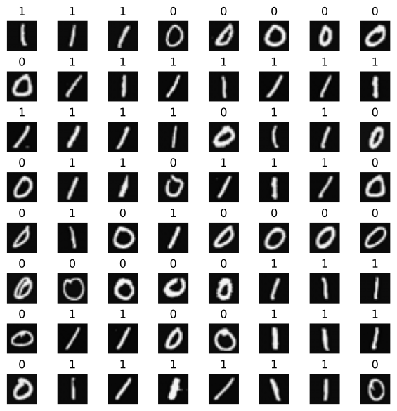
Reshape a row of X back into a 20 by 20 grid to see the actual digit it represents, then display a random selection of 64 images from the dataset, with the true label above each one.
The .T transpose matters here. X[random_index].reshape((20, 20)) fills the grid row by row, left to right, top to bottom, the same unrolling convention used everywhere else on this site. This particular dataset’s images, however, were originally saved filling column by column instead, top to bottom, left to right. Without .T, reshape alone would put every pixel in the wrong spot, and the digit would come out rotated and mirrored rather than upright. .T swaps rows and columns after reshaping, correcting for that.
Review Questions
1. Why does each row of X have exactly 400 entries?
TipAnswer
Each image is \(20 \times 20\) pixels. Unrolled row by row, that gives \(20 \times 20 = 400\) pixel values.
1. How many total training examples are in this dataset, and how are they split between the two digits?
TipAnswer
1000 examples total, 500 of digit 0 and 500 of digit 1.
1. The full downloadable dataset has 5000 images covering all 10 digits. How does X_all[:1000] end up with only zeros and ones?
TipAnswer
The images are stored in blocks by digit, 500 zeros first, then 500 ones, then 500 twos, and so on. The first 1000 rows land exactly on the zero block and the one block.
1. Why does .T matter when reshaping a row of X back into a 20 by 20 image?
TipAnswer
This dataset’s images were originally saved filling the grid column by column, not row by row. reshape alone assumes row-by-row filling, so without .T the digit comes out rotated. .T corrects for that.
Building the Model
Build the same architecture already used for the schematic digit example, a Sequential model with 3 Dense layers, 25 units, then 15, then 1, all with sigmoid activations.
These match the parameter counts in model.summary() exactly, layer 1 alone has over ten thousand parameters, since every one of the 400 pixels connects to all 25 units.
Review Questions
1. Why does layer 1 have so many more parameters than layer 2, even though layer 2 has fewer units too?
TipAnswer
Layer 1 connects 400 input pixels to 25 units, \(400 \times 25 + 25\) parameters. Layer 2 only connects 25 inputs (layer 1’s output) to 15 units, a much smaller \(25 \times 15 + 15\).
Training the Model
Training itself, what compile and fit are actually doing, is covered in detail on a later page. For now, just run it.
model.compile( loss=tf.keras.losses.BinaryCrossentropy(), optimizer=tf.keras.optimizers.Adam(0.001),)history = model.fit(X, y, epochs=20, verbose=0)print("final loss:", history.history["loss"][-1])
final loss: 0.019752968102693558
Making Predictions
Test the trained model on the very first image in the dataset, a 0, and on image 500, the first 1.
prediction = model.predict(X[0].reshape(1, 400), verbose=0)print("predicting a zero:", prediction)prediction = model.predict(X[500].reshape(1, 400), verbose=0)print("predicting a one:", prediction)
predicting a zero: [[0.01429436]]
predicting a one: [[0.9860693]]
The first prediction is close to 0, the second is close to 1, matching the true labels. As before, threshold at 0.5 to get a hard yes-or-no answer.
if prediction >=0.5: yhat =1else: yhat =0print("prediction after threshold:", yhat)
prediction after threshold: 1
Review Questions
1. Why should model.predict on image 0 return a number close to 0, not close to 1?
TipAnswer
Image 0 is a true digit 0. A well-trained model should output a low probability of being a 1 for that image.
Visualizing Predictions
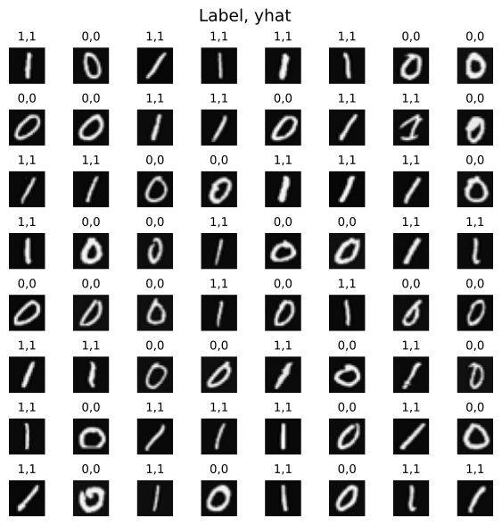
Display another random grid of images, this time showing both the true label and the model’s predicted label above each one.
With this small dataset and only 20 epochs of training, the model gets nearly every image right. Any mismatch between the two numbers in a title is a misclassified digit.
Review Questions
1. In the title above each image, what do the two numbers mean?
TipAnswer
The first number is the true label (\(y\)), the second is the model’s predicted label (\(\hat{y}\)) after thresholding at 0.5.
Summary
In this lab you learned:
A real 20 by 20 pixel digit image unrolls into a 400-number input vector, the same idea used earlier for the smaller schematic 8-by-8 example.
The exact same Sequential, Dense, compile, fit, and predict pattern from the previous pages works unchanged on real image data, only the input size and dataset changed.
Counting a layer’s parameters directly, inputs × units + units, matches what model.summary() reports.
Review Questions
1. What changed about the code compared to the coffee roasting network, and what stayed exactly the same?
TipAnswer
The input size (400 pixels instead of 2 features) and the dataset changed. The Sequential, Dense, compile, fit, and predict pattern itself stayed exactly the same.